from jax import config
config.update("jax_enable_x64", True)
import jax.numpy as jnp
import matplotlib.pyplot as plt

from petitRADTRANS import physics as phys
import numpy as np
from petitRADTRANS.temperature_profiles import guillot_global_temperature_profile
from petitRADTRANS.stellar_spectra.phoenix import PhoenixStarTable

Utility functions

pRT contains some useful utility functions such as a spectral library, pre-implemented pressure-temperature profiles, etc. The use of some of them is shown below. pRT also comes with a package of physical constants, most of which are defined by importing astropy and scipy constants, however.

Constants

Can be accessed by importing import petitRADTRANS.physical_constants as cst. All units are in cgs.

• cst.c: speed of light

• cst.h: Planck constant

• cst.kB: Boltzman constant

• cst.nA: Avogadro constant

• cst.e: electron charge

• cst.G: Gravitational constant

• cst.m_elec: electron mass

• cst.sigma: Stefan-Boltzman constant

• cst.L0: Loschmidt constant

• cst.R: universal gas constant

• cst.bar: 1 bar in cgs

• cst.atm: 1 atmosphere in cgs

• cst.au: Astronomical unit

• cst.pc: parsec

• cst.light_year: light year

• cst.amu: atomic mass unit in g

• cst.r_sun: solar radius

• cst.r_jup: Jupiter equatorial radius

• cst.r_jup_mean: Jupiter mean radius

• cst.r_earth: Earth radius

• cst.m_sun: Solar mass

• cst.m_jup: Jupiter mass

• cst.m_earth: Earth mass

• cst.s_earth: solar_irradiance

Astropy constants (astropy.constants) and scipy constants (scipy.constants) can be directly accessed with cst.a_cst and cst.s_cst, respectively. For example, to get the duration of a year in s: cst.s_cst.year. Caution: constants accessed this way are in SI, not in CGS.

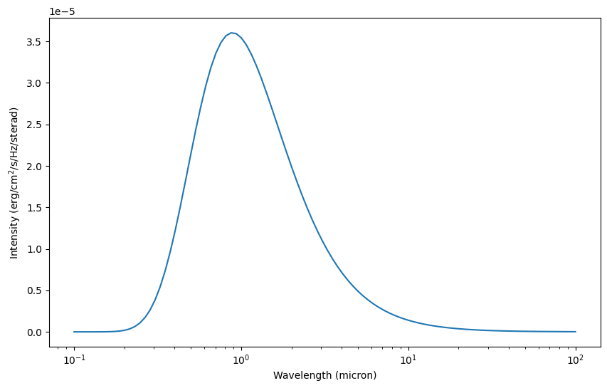
Planck function

The planck function \(B_\nu(T)\), in units of erg/cm\(^2\)/s/Hz/steradian, for a given frequency array, can be generated like this:

# Define wavelength array, in cm
wavelengths_planck = np.logspace(-5, -2, 100)

# Calculate Planck function at 5750 K
planck = phys.planck_function_hz(5750.0, phys.wavelength2frequency(wavelengths_planck))

Let’s plot the Planck function:

# Plot Planck function

plt.rcParams["figure.figsize"] = (10, 6)
plt.plot(wavelengths_planck * 1e4, planck)
plt.xscale("log")
plt.xlabel("Wavelength (micron)")
plt.ylabel("Intensity (erg/cm$^2$/s/Hz/sterad)")

Text(0, 0.5, 'Intensity (erg/cm$^2$/s/Hz/sterad)')

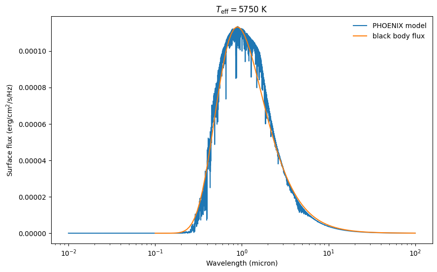
PHOENIX and ATLAS9 stellar model spectra

Within petitRADTRANS the PHOENIX and ATLAS9 stellar spectra can be used, as described in Appendix A of van Boekel et al. (2012). The PHOENIX model refrence, for stellar effective temperatures < 10,000 K is Husser et al. (2013). The ATLAS9 model references for effective temperatures > 10,000 K are Kurucz (1979, 1992, 1994).

The models can be acessed like this, this is for a 5750 K effective temperature star on the main sequence:

star = PhoenixStarTable()
stellar_spec, _ = star.compute_spectrum(5750)
wavelengths = stellar_spec[:, 0]  # (cm)
flux_star = stellar_spec[:, 1]

Loading PHOENIX star table in file '/home/dblain/petitRADTRANS/input_data/stellar_spectra/phoenix/phoenix.startable.petitRADTRANS.h5'... Done.

Let’s plot the spectrum, and also overplot the black body flux from the previous section (note the required factor of \(\pi\) to convert the black body intensity to flux):

plt.plot(wavelengths * 1e4, flux_star, label="PHOENIX model")
plt.plot(wavelengths_planck * 1e4, np.pi * planck, label="black body flux")
plt.title(r"$T_{\rm eff}=5750$ K")
plt.xscale("log")
plt.xlabel("Wavelength (micron)")
plt.ylabel("Surface flux (erg/cm$^2$/s/Hz)")
plt.legend(loc="best", frameon=False)

<matplotlib.legend.Legend at 0x7f18f53e5850>

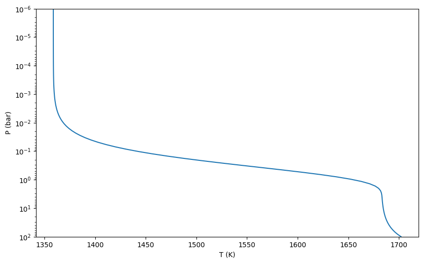
Guillot temperature model

In petitRADTRANS, one can use analytical atmospheric P-T profile from Guillot (2010), his Equation 29: \begin{equation} T^4 = \frac{3T_{\rm int}^4}{4}\left(\frac{2}{3}+\tau\right) + \frac{3T_{\rm equ}^4}{4}\left[\frac{2}{3}+\frac{1}{\gamma\sqrt{3}}+\left(\frac{\gamma}{\sqrt{3}}-\frac{1}{\gamma\sqrt{3}}\right)e^{-\gamma\tau\sqrt{3}}\right] \end{equation} with \(\tau = P\kappa_{\rm IR}/g\). Here, \(\tau\) is the optical depth, \(P\) the pressure, \(\kappa_{\rm IR}\) the atmospheric opacity in the IR wavelengths (i.e. the cross-section per unit mass), \(g\) the atmospheric surface gravity, \(\gamma\) is the ratio between the optical and IR opacity, \(T_{\rm equ}\) the atmospheric equilibrium temperature, and \(T_{\rm int}\) is the planetary internal temperature.

Let’s define an example, all units are cgs units, except for the pressure, which is in bars:

pressures_bar = jnp.logspace(-6, 2, 100)


reference_gravity = 10**3.5

kappa_IR = 0.01

gamma = 0.4

T_int = 200.0

T_equ = 1500.0


temperatures = guillot_global_temperature_profile(
    pressures=pressures_bar,
    infrared_mean_opacity=kappa_IR,
    gamma=gamma,
    gravities=reference_gravity,
    intrinsic_temperature=T_int,
    equilibrium_temperature=T_equ,
)

Let’s plot the P-T profile:

plt.plot(temperatures, pressures_bar)
plt.yscale("log")
plt.ylim([1e2, 1e-6])
plt.xlabel("T (K)")
plt.ylabel("P (bar)")
plt.show()
plt.clf()

<Figure size 1000x600 with 0 Axes>