Retrievals: Basic Retrieval Tutorial#
Written by Evert Nasedkin. Please cite pRT’s retrieval package (Nasedkin et al. 2024) in addition to pRT (Mollière et al. 2019) if you make use of the retrieval package for your work.
How to use these tutorials#
We highly recommend going through all of the various retrieval tutorials! These tutorials are not designed to be copy-and-pasted and used immediately. Rather, we want you to think carefully about the problem you’re solving: what are the modelling choices you need to make, what hardware do you have available, what sampler should you use and so on. Across these tutorials we try to summarize most of the avialable features, but nearly everything can be mixed and matched to set up the best retrieval for your particular problem. If you find something is missing, or there’s a feature you would like added, please reach out and we will try to implement it!
In this tutorial
How to configure and run a retrieval
Setting up parameters
Setting up data
Choosing opacities
Running the retrieval
Generating diagnostic plots
What is a retrieval?#
Let’s start with the basics! An atmospheric retrieval is the process through which we fit a model of a spectrum to data. In the exoplanet community this usually means Bayesian model fitting, for which you can find an introduction here. The model usually incorporates elements of chemistry and radiative transfer in order to compute a spectrum - see the getting started page for an example.
If you’re here, we’re going to assume that you already have an exoplanet emission or transmission spectrum, and you want to learn something about the planet’s properties. We’ll pRT spectral modeling capabilities combined with a sampler which will allow us to statistically measure the properties of the planet of interest. As inputs for this, you’ll need a 1D spectrum with error bars (or a covariance matrix), and a model function that generates a synthetic spectrum. We have a few example datasets included in petitRADTRANS/retrieval/examples/, and several forward models implemented in petitRADTRANS/retrieval/models.py, which you can use directly, or as templates to build your own model. Check out the documentation on the model functions to learn more!These files are included in the pRT package folder. Alternatively you can access them through the git links (just click on the folder / file names above).
In this example we will make use of an HST transmission spectrum, located locally in petitRADTRANS/retrieval/examples/transmission/observations/HST/hst_example_clear_spec.txt, or, again, on git. This dataset is included when you install pRT, and we’ll automatically locate the data and output files throughout the notebook. The outputs of
the retrieval example will be a best-fit spectrum, an atmospheric pressure-temperature profile, and the posterior distributions of all of the parameters of your model atmosphere. Of course, you do not have to use pRT’s retrieval package to run retrievals with pRT-generated spectra, but we believe that what is described below may be sufficient for most people, and will thus save you from most of the tedious implementation work.
Getting started#
You should already have an installation of pRT on your machine; please see the installation manual if you have not installed it yet. Using the [retrieval] or [full] installation will install all of the samplers needed to run any retrieval, though Multinest will also need to be installed separately. Using nested sampling rather than, for example, MCMC is often faster, handles multimodal cases better, and
directly provides the Bayesian evidence, which allows for easier model comparison. Again, see here if you need an introduction to Bayesian model fitting and its terminology. In general, we recommend using JAXNS to start running retrievals. Pymultinest is best suited for running on large CPU clusters. The Hamiltonian Monte Carlo methods work well for high-dimension retrievals, but require more care to set
up, and perform best on GPUs. Please see the sampler documentation to help choose the right sampler for your problem.
In this tutorial, we will outline the process of setting up a RetrievalConfig object, which is the class used to set up a pRT retrieval. The basic process will always be to set up the configuration, and then pass it to the Retrieval class to run the retrieval using pyMultiNest. Several standard plotting outputs will also be produced by the retrieval class. Most of the classes and functions used in this tutorial have more advanced features than what will be explained here, so it’s highly recommended to take a look at the code and API documentation. There should be enough flexibility built in to cover most typical retrieval studies, but if you have feature requests please get in touch, or open an issue on gitlab.
[1]:
# Let's start by importing everything we need.

import os

# To not have numpy start parallelizing on its own when using MPI
os.environ["XLA_FLAGS"] = "--xla_force_host_platform_device_count=2"

# 64-bit precision must be set before importing petitRADTRANS
from jax import config
config.update("jax_enable_x64", True)

# Import the class used to set up the retrieval.
from petitRADTRANS.retrieval import Retrieval, RetrievalConfig
import tensorflow_probability.substrates.jax as tfp

# Import an atmospheric model function
from petitRADTRANS.retrieval.models import isothermal_transmission

# Physical constants
from petitRADTRANS import physical_constants as cst


# Import prior distributions
tfpd = tfp.distributions
Let’s start with a simple model. We’ll use an isothermal temperature profile, and use “free chemistry” - allowing the chemical abundances to vary freely within fixed boundaries, but requiring them to be vertically constant throughout the atmosphere. The basic process for every retrieval will be the same. We need to set up a RetrievalConfig object, adding in the Data objects that we want to fit together with the Parameter objects and their priors, which we can use to customize our retrieval.
Retrieval configuration object and parameters#
Let’s start out by setting up a simple run definition. We’ll add the data AFTER we define the model function below. We start out by initialising the RetrievalConfig object (which we call retrieval_config here), and then adding each of the parameters of interest to it.
Each parameter must be given a name, which matches the name used in the model function defined below. Parameters can be set to fixed or free. Fixed parameters must be given a value, while free parameters are given a function that transforms the unit hypercube generated by multinest into physical prior space. Various prior functions are stored in retrieval.utils, see the API documentation. Full details of the parameters can be found
in the API documentation.
[2]:
# Lets start out by setting up a simple run definition
# We'll add the data AFTER we define the model function below
# Full details of the parameters can be found in retrieval_config.py

# If our retrieval has already run before, you can set the run_mode to 'evaluate' to only make some plots.
retrieval_config = RetrievalConfig(
    retrieval_name="hst_example_clear_spec",
    run_mode="retrieval",  # this can be 'evaluate' to get the results of a retrieval
    sampler_type="jaxns",  # The sampler to use. Here we use the JAXNS sampler.
    adaptive_mesh_refinement=False,  # We won't be using adaptive mesh refinement for the pressure grid
    # This would turn on scattering when calculating emission spectra (always activated in transmission).
    scattering_in_emission=False,
)

# Let's start with the parameters that will remain fixed during the retrieval
retrieval_config.add_parameter(
    name="stellar_radius",  # name
    is_free_parameter=False,  # is_free_parameter, so stellar_radius is not retrieved here.
    value=0.651 * cst.r_sun,
    plot_in_corner=False,  # we won't be plotting this parameter in the corner plot
)

# Log of the surface gravity in cgs units.
# The transform_prior_cube_coordinate function transforms a uniform random sample x, drawn between 0 and 1.
# to the physical units we're using in pRT. We use Python's lambda functions here.
retrieval_config.add_parameter(
    name="log_g",
    is_free_parameter=True,  # is_free_parameter: we are retrieving log(g) here
    distribution=tfpd.Uniform(low=2.0, high=5.5),  # this means that log g can vary between 2 and 5.5
    plot_in_corner=True,  # we will plot this parameter in the corner plot
    corner_ranges=(2.0, 5.5),  # this sets the range of the axis in the corner plot
    corner_label=r"$\log(g)$",  # this sets the label of the axis in the corner plot
)
# Note that logg is usually not a free parameter in retrievals of
# transmission spectra, at least it is much better constrained as being
# assumed here, as the planetary mass and radius are usually known.

# Planet radius in cm
retrieval_config.add_parameter(
    name="planet_radius",
    is_free_parameter=True,
    distribution=tfpd.Uniform(low=0.1 * cst.r_jup, high=0.4 * cst.r_jup),  # radius varies between 0.2 and 0.4 R_jup
    plot_in_corner=True,  # we will plot this parameter in the corner plot
    corner_ranges=(0.1, 0.4),  # this sets the range of the axis in the corner plot
    corner_label=r"R$_{pl}$",  # this sets the label of the axis in the corner plot
    corner_transform=lambda x: x / cst.r_jup_mean,  # this transforms the units in the corner plot to R_jup
)

# Atmospheric temperature in Kelvin
retrieval_config.add_parameter(
    name="temperature",
    is_free_parameter=True,
    distribution=tfpd.Uniform(low=300, high=2000),
    plot_in_corner=True,  # we will plot this parameter in the corner plot
    corner_ranges=(300, 2000),  # this sets the range of the axis in the corner plot
    corner_label=r"Temp",  # this sets the label of the axis in the corner plot
)

# Let's include a grey cloud as well to see what happens, even though we assumed a clear atmosphere.
retrieval_config.add_parameter(
    "log_Pcloud",
    is_free_parameter=True,
    distribution=tfpd.Uniform(low=-6, high=2),  # the atmosphere can have an opaque cloud between 1e-6 and 100 bar
    plot_in_corner=True,  # we will plot this parameter in the corner plot
    corner_ranges=(-6, 2),  # this sets the range of the axis in the corner plot
    corner_label=r"$\log P_{cl}$",  # this sets the label of the axis in the corner plot
)
Opacities#
petitRADTRANS can be setup to use line-by-line opacities at \(\lambda/\Delta \lambda = 10^6\), or a lower resolution correlated-k mode (which we use here). The names of each species must follow the naming convention explained here, which also contains a list of available species. ‘Getting Started’ also has an example for how to load opacities in pRT.
In addition to line opacities, pRT can also include, for example, Rayleigh scattering, collision-induced absorption (CIA) opacities, or opacities for various condensate cloud species. Again, see here for a list. If a cloud species is used, it will have a set of parameters added in order to retrieve the cloud abundance. We give such an example below. The parameters added depend on the model chosen.
If you aren’t sure which species are available, the RetrievalConfig class has a few functions that will list the currently available line, CIA and cloud opacities, see the API documentation.
Opacity resolution#
Do not append resolution identifiers, for example .R100, to the species name, if you want to use a correlated-k species at lower resolution of \(\lambda/\Delta \lambda = 100\), instead of the nominal \(\lambda/\Delta \lambda = 1000\). Instead, you will specify a model resolution when adding data (see below). If you set the model resolution for your data, and do not have existing c-k tables at that resolution,
Exo_k will be used to bin the higher resolution tables down to a lower resolution. Please cite Exo_k and the corresponding paper (Leconte et al. 2021) if you make use of this functionality in pRT.
You can use retrieval_config.list_available_line_species() to see which line species are available on your machine, but note that pRT will automatically download those listed here if you request some that you do not have yet.
Let’s add some opacities below now:
[3]:
retrieval_config.set_rayleigh_species(["H2", "He"])
retrieval_config.set_continuum_opacities(["H2--H2", "H2--He"])

# Here we setup the line species for a free retrieval,
# setting the prior bounds of the log10 abundance with the abund_lim parameter
# So the retrieved value is the log mass fraction.
retrieval_config.set_line_species(
    ["1H2-16O__POKAZATEL", "12C-1H4__HITEMP", "12C-16O2__UCL-4000", "C-O-NatAbund__HITEMP"],
    use_equilibrium_chemistry=False,
    free_mass_fraction_limits=(-6.0, 0.0),
    plot_in_corner=True,
)
Model Functions#
In addition to setting up a retrieval with a standard model, you may also want to write your own model to be used in the retrieval setup, as shown in the model function documentation.. For this example we will use the built-in isothermal_transmission model.
Data#
With the model set up, we can read in the data. The data must be a 1D spectrum with error bars or a covariance matrix. The input format for ASCII data is
# Wavelength [micron], Flux [W/m2/micron or (Rp/Rstar)^2], Flux Error [W/m2/micron or (Rp/Rstar)^2]
Optionally, there can also be an additional column to specify the wavelength bins, which would then have the format:
# Wavelength [micron], Bins [micron], Flux [W/m2/micron or (Rp/Rstar)^2], Flux Error [W/m2/micron or (Rp/Rstar)^2]
The file can be comma or space separated, and by default ‘#’ is the comment character. The wavelength column must be sorted and is in ascending order. If you write your own model function, the units of your data can vary from this template, but the units of your data and the output of your model function must match. Throughout our documentation we will use W/m^2/micron for emission spectra and (Rp/Rstar)^2 for consistency between our model functions and the example data.
The fits file requirements are more strict. An extension labelled ‘SPECTRUM’ is required, with three fields in a binary table: ‘WAVELENGTH’, ‘FLUX’ and ‘COVARIANCE’. An example of this is the HR8799e_spectra.fits file included in petitRADTRANS/retrieval/examples/emission/, see pRT’s gitlab page. If your file is not of that format, but you want to
add a covariance matrix, you could also fill in these attributes of the data object that gets added to the retrieval configuration after calling add_data():
covariance: the covariance matrixinv_cov: the inverse of the covariance matrixlog_covariance_determinant: the natural logarithm of the derterminant of the covariance matrix
The Data class is arguably the most important part of setting up the retrieval. Not only do you input your data here, but you also choose your model function and resolution. This means that you can design a retrieval around different datatypes and retrieve simultaneously on both - for example, if you want the day and nightside of a planet, or want to combine the eastward and westward limbs of a transmission spectrum with different models.
By adjusting the resolution you can also speed up the retrieval. By default, pRT uses the correlated-k method for computing opacities, which works up to \(\lambda/\Delta \lambda = 1000\). Here you need to pick 'c-k' as line_opacity_mode, see below. Often low resolution data does not require this resolution, and the computation can be sped up using the model_resolution parameter, which will use the Exo-k package to bin down the correlated-k tables.
If you use the 'lbl' (line-by-line) mode, pRT can uses opacities up to \(\lambda/\Delta \lambda = 10^6\), though this is quite slow and memory intensive. By setting the model_resolution parameter, pRT will sample the high resolution line list at the specified resolution (e.g., model_resolution=10**5. will down-sample by a factor of 10). In this case you must make sure that the down-sampled calculations match the binned-down results of the \(\lambda/\Delta \lambda = 10^6\)
mode at the required data resolution (i.e., sampling can introduce noise and you have to test for that).
The Data class can also handle photometric data, which is described in the emission tutorial.
[4]:
# Finally, we associate the model with the data, and we can run our retrieval!

# Here we import petitRADTRANS to find the path of the example files on your machine.
# In general this is not required, you just put the files in the folder that you are running
# Your script in, for example.

path_to_data = "./"  # Default location for the example
retrieval_config.add_data(
    name="HST",  # simulated HST data
    path_to_observations=f"{path_to_data}retrievals/transmission/observations/HST/hst_example_clear_spec.txt",  # where is the data
    model_generating_function=isothermal_transmission,  # the atmospheric model to use
    line_opacity_mode="c-k",
    data_resolution=60,  # the spectral resolution of the data
    model_resolution=120,  # the resolution of the c-k tables for the lines
)
# This model is a noise-free, clear atmosphere transmission spectrum for a sub-neptune type planet
# The model function used to calculate it was slightly different, and used different opacity tables
# than what we'll use in the retrieval, but the results don't significantly change.
# You could even see it as a simulation of reality since we never have the perfect model or opacities
# that "Nature" is using.
#
# In general, it is also necessary to use the data_resolution and model_resolution arguments.
# The data_resolution argument will convolve the generated model spectrum by the instrumental
# resolution before to calculating the chi squared value. As mentioned at the bottom of
# "Rebinning opacities", the model resolution should be >= 2 times larger than the data resolution.
#
# The model_resolution parameter will cause pRT to use exo-k to generate low-resolution correlated-k opacity tables
# in order to speed up the radiative transfer calculations (if this has not been done yet).
Plotting#
Let’s also set up some plotting details so that we can generate nice outputs after the retrieval has finished.
Each parameter can be added to the corner plot, its label changed, and the values transformed to more digestible units (e.g., the planet radius in jupiter radii, rather than cm). We can also set the bounds and scaling on the best-fit spectrum plot and the limits for the P-T profile plot. With this complete, our retrieval is ready to go.
Most parameters include a default setting, so the plots will be created even if you don’t set any plotting parameters, but the outputs might not be very informative. In general, the possible arguments to plot_kwargs follow the naming conventions of matplotlib arguments and functions, with some additions. Full details of the plotting can be found in the Retrieval class, see the API documentation.
[5]:
# Define axis properties of spectral plot if run_mode == 'evaluate'

def configure_retrieval_plotter(retrieval):
    retrieval.plotter.spec_xlabel = "Wavelength [micron]"
    retrieval.plotter.spec_ylabel = "Transit Depth [ppm]"
    retrieval.plotter.y_axis_scaling = 1e6
    retrieval.plotter.xscale = "linear"
    retrieval.plotter.yscale = "linear"
    retrieval.plotter.resolution = None  # maximum resolution, will rebin the data
    # Define from which observation object to take P-T in evaluation mode.
    retrieval.plotter.reference_data_name = "HST"
    retrieval.plotter.temp_limits = [150, 3000]
    retrieval.plotter.press_limits = [1e2, 1e-5]

# If in doubt, define all of the plot_kwargs used here.
Running the retrieval#
At this point, we are almost ready to run the retrieval! We only need to do is pass the RunDefinition object “retrieval_config” we just created to an object of the Retrieval class first.
[6]:
output_directory = "./retrievals/runs"

retrieval = Retrieval(
    configuration=retrieval_config,
    output_directory=output_directory,
    evaluate_sample_spectra=False,
    use_prt_plot_style=True,
)
Setting up Radtrans object for data 'HST'...
Loading Radtrans opacities...
 Loading line opacities of species '1H2-16O__POKAZATEL.R120' from file '/Users/nasedkin/python-packages/petitRADTRANS/input_data/opacities/lines/correlated_k/H2O/1H2-16O/1H2-16O__POKAZATEL.R120_0.3-50mu.ktable.petitRADTRANS.h5'... Done.
 Loading line opacities of species '12C-1H4__HITEMP.R120' from file '/Users/nasedkin/python-packages/petitRADTRANS/input_data/opacities/lines/correlated_k/CH4/12C-1H4/12C-1H4__HITEMP.R120_0.1-250mu.ktable.petitRADTRANS.h5'... Done.
 Loading line opacities of species '12C-16O2__UCL-4000.R120' from file '/Users/nasedkin/python-packages/petitRADTRANS/input_data/opacities/lines/correlated_k/CO2/12C-16O2/12C-16O2__UCL-4000.R120_0.3-50mu.ktable.petitRADTRANS.h5'... Done.
 Loading line opacities of species 'C-O-NatAbund__HITEMP.R120' from file '/Users/nasedkin/python-packages/petitRADTRANS/input_data/opacities/lines/correlated_k/CO/C-O-NatAbund/C-O-NatAbund__HITEMP.R120_0.1-250mu.ktable.petitRADTRANS.h5'... Done.
 Successfully loaded all line opacities
 Loading CIA opacities for H2--H2 from file '/Users/nasedkin/python-packages/petitRADTRANS/input_data/opacities/continuum/collision_induced_absorptions/H2--H2/H2--H2-NatAbund/H2--H2-NatAbund__BoRi.R831_0.6-250mu.ciatable.petitRADTRANS.h5'... Done.
 Loading CIA opacities for H2--He from file '/Users/nasedkin/python-packages/petitRADTRANS/input_data/opacities/continuum/collision_induced_absorptions/H2--He/H2--He-NatAbund/H2--He-NatAbund__BoRi.DeltaWavenumber2_0.5-500mu.ciatable.petitRADTRANS.h5'... Done.
 Successfully loaded all CIA opacities
Successfully loaded all opacities
[7]:
configure_retrieval_plotter(retrieval)
Now, we can call the retrieval.run() method and run the retrieval!
There are a few additional parameters that can be adjusted, but the defaults should work well for almost all use cases. In general it may not be wise to run a retrieval on your laptop, as it can be quite computationally expensive. However, the included HST example should be able to be run fairly easily! (minutes!). We only use 80 live points in the example so that it runs in a reasonable length of time, but we highly recommend using more live points for your own retrievals! For JAXNS we’s also
recommended to tighten the termination conditions in order to obtain better fits during retrievals, as described in the sampler documentation. If you want to run the retrieval on a cluster, or just on multiple cores on your local machine, see the documentation on retrieval parallelisation. Most of the various parameters used to control pyMultiNest or Ultranest can be set in the retrieval.run() function, see the API
documentation.
[ ]:
retrieval.run(
    num_live_points=40,
    max_samples=1e5,
    verbose=True,
    parameter_estimation=True,
)
Starting retrieval hst_example_clear_spec with jaxns
Testing data 'HST':
 wavelengths:
  OK (no NaN, infinite, or negative value detected)
 spectrum:
  OK (no NaN, infinite, or negative value detected)
 uncertainties:
  OK (no NaN, infinite, or negative value detected)
Testing model function for data 'HST'...
No errors detected in the model functions!
INFO:jaxns:Number of Markov-chains set to: 40
Running over 2 devices.
Starting JAXNS retrieval: hst_example_clear_spec
Creating initial state with 40 live points.
Running uniform sampling down to efficiency threshold of 0.05.
Running until termination condition: TerminationCondition(ess=None, evidence_uncert=None, live_evidence_frac=None, dlogZ=None, max_samples=Array(100000, dtype=int64), max_num_likelihood_evaluations=None, log_L_contour=None, efficiency_threshold=None, rtol=None, atol=None, peak_XL_frac=Array(0.1, dtype=float64))
-------
Num samples: 20
Num likelihood evals: 763
Efficiency: 0.05108556832694764
log(L) contour: -6892.749624646676
log(Z) est.: 128.22558729946167 +- 0.7970341919152178
log(Z | remaining) est.: 7026.191268726718 +- 1.1470044861628728
ESS: 0.5557768160623715
-------
Num samples: 40
Num likelihood evals: 1561
Efficiency: 0.03389830508474576
log(L) contour: -1105.2961305128724
log(Z) est.: 128.39747026421173 +- 0.6877213173513662
log(Z | remaining) est.: 1239.4094604195839 +- 1.0794524624834452
ESS: 0.8264008778101513
-------
Num samples: 60
Num likelihood evals: 2516
Efficiency: 0.027416038382453736
log(L) contour: -247.26713727546857
log(Z) est.: 141.79056077640107 +- 0.6977436879768433
log(Z | remaining) est.: 395.2733605559853 +- 1.0913315182091228
ESS: 0.8123441250659745
-------
Num samples: 80
Num likelihood evals: 3692
Efficiency: 0.021413276231263382
log(L) contour: 19.077562622481878
log(Z) est.: 142.67976991653134 +- 0.702775103960175
log(Z | remaining) est.: 130.31767266031386 +- 1.0999783159634513
ESS: 0.8131441078788413
-------
Num samples: 100
Num likelihood evals: 5118
Efficiency: 0.018042399639152006
log(L) contour: 102.02573242285189
log(Z) est.: 142.1823021616678 +- 0.710333452007959
log(Z | remaining) est.: 47.326456304726364 +- 1.099304427966011
ESS: 0.8061444239777501
-------
Num samples: 120
Num likelihood evals: 7040
Efficiency: 0.013063357282821686
log(L) contour: 129.46991232218565
log(Z) est.: 141.68955027430854 +- 0.7160689534560669
log(Z | remaining) est.: 18.437202170721008 +- 0.914972144839323
ESS: 0.8045851855722707
-------
Num samples: 140
Num likelihood evals: 9198
Efficiency: 0.010875475802066341
log(L) contour: 132.5202788190748
log(Z) est.: 141.4410753093405 +- 0.6448549460370167
log(Z | remaining) est.: 14.099482649239135 +- 0.730295787949944
ESS: 1.0997685999678257
-------
Num samples: 160
Num likelihood evals: 11467
Efficiency: 0.009852216748768473
log(L) contour: 134.2711589394577
log(Z) est.: 152.95490746595908 +- 0.8742123341718354
log(Z | remaining) est.: 23.687865559716556 +- 0.9304426171569603
ESS: 0.4656900385488618
-------
Num samples: 180
Num likelihood evals: 13871
Efficiency: 0.009029345372460496
log(L) contour: 138.77375345670228
log(Z) est.: 157.962156015528 +- 0.8786273951866798
log(Z | remaining) est.: 26.398301819727976 +- 0.992568459789689
ESS: 0.4640355615113089
-------
Num samples: 200
Num likelihood evals: 16663
Efficiency: 0.008238928939237899
log(L) contour: 145.11153789057357
log(Z) est.: 159.20106483123783 +- 0.7017151699550143
log(Z | remaining) est.: 21.98671861428005 +- 0.8564819250224457
ESS: 0.9316533185423133
-------
Num samples: 220
Num likelihood evals: 19526
Efficiency: 0.007311277645768598
log(L) contour: 148.88376642654444
log(Z) est.: 158.81689527744246 +- 0.6736817179486919
log(Z | remaining) est.: 17.52076542410839 +- 0.8130849472696643
ESS: 1.0831235765231573
-------
Num samples: 240
Num likelihood evals: 22352
Efficiency: 0.007293946024799417
log(L) contour: 154.5068485528743
log(Z) est.: 158.41070790967265 +- 0.653431384915346
log(Z | remaining) est.: 12.317762791873946 +- 0.821990082685915
ESS: 1.2298327452668825
-------
Num samples: 260
Num likelihood evals: 25613
Efficiency: 0.0068073519400953025
log(L) contour: 158.16822444249559
log(Z) est.: 158.4616460773778 +- 0.5762077745596047
log(Z | remaining) est.: 8.91423389933783 +- 0.7317852729012342
ESS: 1.9666247430966548
-------
Num samples: 280
Num likelihood evals: 28969
Efficiency: 0.006379585326953748
log(L) contour: 162.18096889305428
log(Z) est.: 160.77687482879085 +- 0.784240682122516
log(Z | remaining) est.: 7.942460603790181 +- 0.9229073954300052
ESS: 0.7178284892313149
-------
Num samples: 300
Num likelihood evals: 32377
Efficiency: 0.006192909119058678
log(L) contour: 164.29625518012062
log(Z) est.: 160.86694994430178 +- 0.6301892176331556
log(Z | remaining) est.: 5.592702249558073 +- 0.7720499575763752
ESS: 1.5594599504686346
-------
Num samples: 320
Num likelihood evals: 35984
Efficiency: 0.005928560841855639
log(L) contour: 166.02128675988175
log(Z) est.: 161.40141718498867 +- 0.5608074270608555
log(Z | remaining) est.: 4.661480793206692 +- 0.7111438629269892
ESS: 2.648381283435282
-------
Num samples: 340
Num likelihood evals: 39558
Efficiency: 0.005865102639296188
log(L) contour: 167.56310665826882
log(Z) est.: 161.35287035513022 +- 0.5112192500870159
log(Z | remaining) est.: 3.237204240167074 +- 0.6788834740014529
ESS: 4.79072367008182
-------
Num samples: 360
Num likelihood evals: 43326
Efficiency: 0.005593623269472801
log(L) contour: 168.866900194218
log(Z) est.: 161.62268388149846 +- 0.48174024399680876
log(Z | remaining) est.: 2.4790028688500456 +- 0.6576410341129786
ESS: 9.27188271845339
-------
Num samples: 380
Num likelihood evals: 47227
Efficiency: 0.005341880341880342
log(L) contour: 169.6468014537022
log(Z) est.: 161.66966528643502 +- 0.4717148401783954
log(Z | remaining) est.: 1.7223566720541328 +- 0.6526725010901341
ESS: 16.219746317624374
-------
Num samples: 400
Num likelihood evals: 51396
Efficiency: 0.005061369100341643
log(L) contour: 170.66414446055978
log(Z) est.: 161.71539443752278 +- 0.46916966955254047
log(Z | remaining) est.: 1.1440739659124972 +- 0.6541766128844486
ESS: 26.129687549794635
-------
Num samples: 420
Num likelihood evals: 56071
Efficiency: 0.004724781478856603
log(L) contour: 171.2071564488269
log(Z) est.: 161.75540727983025 +- 0.46890940374944423
log(Z | remaining) est.: 0.732844846496647 +- 0.6565720364598959
ESS: 38.60137485840067
-------
Num samples: 440
Num likelihood evals: 60835
Efficiency: 0.004543389368468878
log(L) contour: 171.57604101420822
log(Z) est.: 161.78114545530903 +- 0.4692097273828878
log(Z | remaining) est.: 0.4685404931940411 +- 0.6586013788596571
ESS: 50.92798984203019
-------
Num samples: 460
Num likelihood evals: 65681
Efficiency: 0.004438033950959725
log(L) contour: 171.73152043508819
log(Z) est.: 161.7975692165729 +- 0.46953629807594566
log(Z | remaining) est.: 0.2997380185164502 +- 0.6603015924340498
ESS: 60.55120886998844
-------
Num samples: 480
Num likelihood evals: 70661
Efficiency: 0.004306168586500162
log(L) contour: 171.9315072797032
log(Z) est.: 161.80589566843298 +- 0.4697240263404712
log(Z | remaining) est.: 0.19118268603273236 +- 0.661586084391458
ESS: 66.75524322088306
-------
Num samples: 500
Num likelihood evals: 76070
Efficiency: 0.003915426781519186
log(L) contour: 172.02667607404277
log(Z) est.: 161.81072240118385 +- 0.46984405755253766
log(Z | remaining) est.: 0.12053791353213228 +- 0.6625733387666134
ESS: 70.11151989680745
-------
Num samples: 520
Num likelihood evals: 81566
Efficiency: 0.003766833035125718
log(L) contour: 172.12089079810863
log(Z) est.: 161.8134021115634 +- 0.4699140487688145
log(Z | remaining) est.: 0.07625683085768742 +- 0.6632698410437547
ESS: 71.76218435328983
-------
Num samples: 540
Num likelihood evals: 87451
Efficiency: 0.0035932446999640674
log(L) contour: 172.18194537219614
log(Z) est.: 161.8146583123553 +- 0.4699476875891617
log(Z | remaining) est.: 0.04743635499295351 +- 0.6637573343759038
ESS: 72.50635058614364
-------
Num samples: 560
Num likelihood evals: 93193
Efficiency: 0.0035279590756747223
log(L) contour: 172.21751690613772
log(Z) est.: 161.81519091090814 +- 0.4699620940395432
log(Z | remaining) est.: 0.029243756999306925 +- 0.6640811592248016
ESS: 72.81835423563169
--------
Termination Conditions:
XL < max(XL) * peak_XL_frac
--------
likelihood evals: 93233
samples: 600
phantom samples: 0
likelihood evals / sample: 155.4
phantom fraction (%): 0.0%
--------
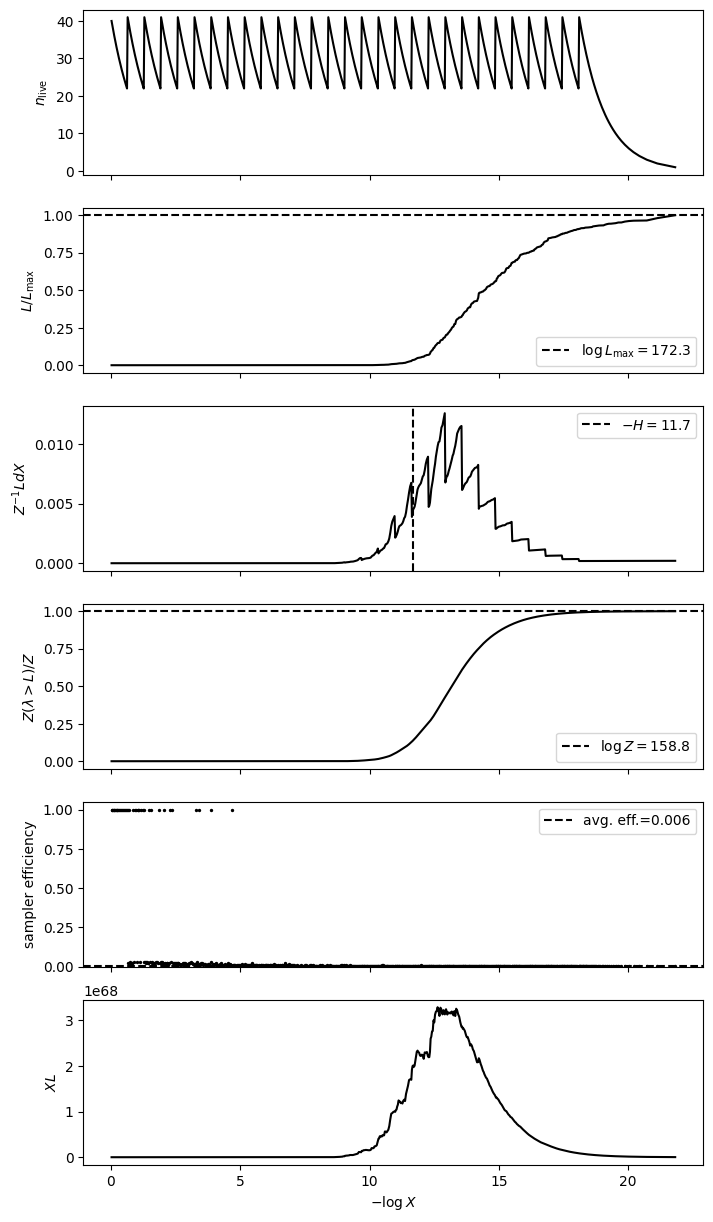
logZ=158.81 +- 0.61
max(logL)=172.31
H=-11.66
ESS=53
--------
12C-16O2__UCL-4000: mean +- std.dev. | 10%ile / 50%ile / 90%ile | MAP est. | max(L) est.
12C-16O2__UCL-4000: -4.14 +- 0.96 | -5.64 / -3.95 / -3.0 | -3.79 | -3.79
--------
12C-1H4__HITEMP: mean +- std.dev. | 10%ile / 50%ile / 90%ile | MAP est. | max(L) est.
12C-1H4__HITEMP: -2.1 +- 0.41 | -2.55 / -2.11 / -1.66 | -2.36 | -2.36
--------
1H2-16O__POKAZATEL: mean +- std.dev. | 10%ile / 50%ile / 90%ile | MAP est. | max(L) est.
1H2-16O__POKAZATEL: -2.0 +- 0.35 | -2.5 / -1.99 / -1.65 | -2.13 | -2.13
--------
C-O-NatAbund__HITEMP: mean +- std.dev. | 10%ile / 50%ile / 90%ile | MAP est. | max(L) est.
C-O-NatAbund__HITEMP: -4.4 +- 1.2 | -5.5 / -4.9 / -2.7 | -5.1 | -5.1
--------
log_Pcloud: mean +- std.dev. | 10%ile / 50%ile / 90%ile | MAP est. | max(L) est.
log_Pcloud: -0.76 +- 1.0 | -2.12 / -0.82 / 0.74 | -0.05 | -0.05
--------
log_g: mean +- std.dev. | 10%ile / 50%ile / 90%ile | MAP est. | max(L) est.
log_g: 2.993 +- 0.062 | 2.915 / 3.001 / 3.056 | 3.005 | 3.005
--------
planet_radius: mean +- std.dev. | 10%ile / 50%ile / 90%ile | MAP est. | max(L) est.
planet_radius: 1193000000.0 +- 71000000.0 | 1099000000.0 / 1198000000.0 / 1284000000.0 | 1222000000.0 | 1222000000.0
--------
temperature: mean +- std.dev. | 10%ile / 50%ile / 90%ile | MAP est. | max(L) est.
temperature: 850.0 +- 120.0 | 720.0 / 870.0 / 970.0 | 870.0 | 870.0
--------
{'samples': array([[ 3.00522132e+00,  1.22178673e+09,  8.70568870e+02, ...,
         -2.35928246e+00, -3.78508470e+00, -5.05384181e+00],
        [ 2.91545576e+00,  1.17336856e+09,  7.29833801e+02, ...,
         -2.32278208e+00, -4.70258384e+00, -2.94178948e+00],
        [ 2.89498825e+00,  1.08805622e+09,  7.72032524e+02, ...,
         -2.53416077e+00, -3.66842177e+00, -5.43607514e+00],
        ...,
        [ 2.85958715e+00,  1.18507625e+09,  6.95272558e+02, ...,
         -2.26902010e+00, -4.01338931e+00, -5.68031277e+00],
        [ 2.93902133e+00,  1.20926118e+09,  7.21437201e+02, ...,
         -1.90617892e+00, -5.08913179e+00, -3.26769376e+00],
        [ 3.02499658e+00,  1.25620822e+09,  8.09237887e+02, ...,
         -1.93871484e+00, -3.39688049e+00, -4.73286695e+00]]),
 'log_likelihood': array([172.31267101, 170.5304988 , 170.53855608, 171.35221085,
        172.00776274, 170.40996731, 168.15802924, 171.67215047,
        172.01921348, 171.16826826, 171.51221265, 169.08852486,
        169.67227287, 167.54606565, 171.66670295, 169.9364714 ,
        170.94377795, 170.5304988 , 171.80449684, 171.61676028,
        169.54130574, 171.82653958, 171.30874729, 170.66414446,
        171.51221265, 171.71299725, 171.82839607, 170.16204548,
        167.8119149 , 172.01921348, 169.9364714 , 168.71993336,
        166.59781303, 170.94377795, 170.40847118, 170.95514075,
        171.69641824, 171.13194458, 171.1061656 , 171.58668222,
        172.0179844 , 171.87397819, 170.70976822, 168.6817075 ,
        167.8119149 , 171.465609  , 170.24935553, 169.23962332,
        171.95495424, 171.40767629, 172.18783102, 172.16075981,
        170.39813185, 170.53855608, 170.72054177, 171.01801384,
        171.2429024 , 169.35808576, 170.94377795, 171.17006963,
        172.09573578, 171.93016404, 171.93016404, 170.95514075,
        171.36213336, 171.16826826, 171.35221085, 169.29922962,
        170.62532245, 171.84916097, 169.32881946, 172.20884363,
        171.18095985, 170.62532245, 169.67227287, 171.78975787,
        169.62960831, 171.34070522, 171.73152044, 171.57604101,
        172.09573578, 170.40847118, 171.16826826, 166.6248844 ,
        170.39813185, 169.54130574, 170.53855608, 171.82877089,
        170.5304988 , 171.01801384, 171.71299725, 172.07371216,
        166.20886786, 172.04370731, 171.71299725, 169.32314076,
        171.16826826, 171.30874729, 171.51221265, 169.57706419,
        171.34070522, 167.99539784, 171.57604101, 172.2224413 ,
        171.18095985, 170.62532245, 170.3395356 , 170.94377795,
        171.73152044, 167.8119149 , 171.79577892, 170.40847118,
        171.59815959, 172.03953008, 170.78986991, 169.74817476,
        170.72437065, 170.24935553, 171.58668222, 170.91690713,
        170.61026372, 171.36213336, 170.61026372, 171.59705614,
        168.41536461, 169.74817476, 172.06415002, 169.62960831,
        171.57604101, 171.67339964, 170.00535414, 171.87941868,
        171.25994195, 171.7315136 , 171.1061656 , 171.4268204 ,
        171.79828274, 172.02667607, 172.15226123, 171.43265948,
        171.16826826, 172.25452936, 171.17006963, 171.45397976,
        168.31216898, 169.29922962, 170.81549201, 171.71299725,
        171.6908012 , 168.6817075 , 171.17006963, 171.13194458,
        171.13194458, 167.56310666, 170.3395356 , 170.72437065]),
 'log_weights': array([-5.04985601, -5.04985601, -5.04985601, -5.04985601, -5.04985601,
        -5.04985601, -5.04985601, -5.04985601, -5.04985601, -5.04985601,
        -5.04985601, -5.04985601, -5.04985601, -5.04985601, -5.04985601,
        -5.04985601, -5.04985601, -5.04985601, -5.04985601, -5.04985601,
        -5.04985601, -5.04985601, -5.04985601, -5.04985601, -5.04985601,
        -5.04985601, -5.04985601, -5.04985601, -5.04985601, -5.04985601,
        -5.04985601, -5.04985601, -5.04985601, -5.04985601, -5.04985601,
        -5.04985601, -5.04985601, -5.04985601, -5.04985601, -5.04985601,
        -5.04985601, -5.04985601, -5.04985601, -5.04985601, -5.04985601,
        -5.04985601, -5.04985601, -5.04985601, -5.04985601, -5.04985601,
        -5.04985601, -5.04985601, -5.04985601, -5.04985601, -5.04985601,
        -5.04985601, -5.04985601, -5.04985601, -5.04985601, -5.04985601,
        -5.04985601, -5.04985601, -5.04985601, -5.04985601, -5.04985601,
        -5.04985601, -5.04985601, -5.04985601, -5.04985601, -5.04985601,
        -5.04985601, -5.04985601, -5.04985601, -5.04985601, -5.04985601,
        -5.04985601, -5.04985601, -5.04985601, -5.04985601, -5.04985601,
        -5.04985601, -5.04985601, -5.04985601, -5.04985601, -5.04985601,
        -5.04985601, -5.04985601, -5.04985601, -5.04985601, -5.04985601,
        -5.04985601, -5.04985601, -5.04985601, -5.04985601, -5.04985601,
        -5.04985601, -5.04985601, -5.04985601, -5.04985601, -5.04985601,
        -5.04985601, -5.04985601, -5.04985601, -5.04985601, -5.04985601,
        -5.04985601, -5.04985601, -5.04985601, -5.04985601, -5.04985601,
        -5.04985601, -5.04985601, -5.04985601, -5.04985601, -5.04985601,
        -5.04985601, -5.04985601, -5.04985601, -5.04985601, -5.04985601,
        -5.04985601, -5.04985601, -5.04985601, -5.04985601, -5.04985601,
        -5.04985601, -5.04985601, -5.04985601, -5.04985601, -5.04985601,
        -5.04985601, -5.04985601, -5.04985601, -5.04985601, -5.04985601,
        -5.04985601, -5.04985601, -5.04985601, -5.04985601, -5.04985601,
        -5.04985601, -5.04985601, -5.04985601, -5.04985601, -5.04985601,
        -5.04985601, -5.04985601, -5.04985601, -5.04985601, -5.04985601,
        -5.04985601, -5.04985601, -5.04985601, -5.04985601, -5.04985601,
        -5.04985601]),
 'weighted_samples': {'points': array([[ 2.18819834e+00,  2.38329197e+09,  8.78646136e+02, ...,
          -4.08693804e+00, -6.04271296e-01, -1.99074577e+00],
         [ 2.09268753e+00,  2.24976970e+09,  1.05016700e+03, ...,
          -5.68881265e+00, -3.43467393e+00, -3.96064262e+00],
         [ 2.01491024e+00,  2.19048620e+09,  5.97941648e+02, ...,
          -3.65308736e+00, -4.16359450e+00, -1.06016428e+00],
         ...,
         [ 2.99654154e+00,  1.23332446e+09,  8.39862622e+02, ...,
          -2.35313124e+00, -3.84729194e+00, -5.06713322e+00],
         [ 3.01740928e+00,  1.21056493e+09,  8.90232579e+02, ...,
          -2.24378830e+00, -3.85503517e+00, -5.02401574e+00],
         [ 3.00522132e+00,  1.22178673e+09,  8.70568870e+02, ...,
          -2.35928246e+00, -3.78508470e+00, -5.05384181e+00]]),
  'logl': array([-1.01331902e+12, -3.82621150e+11, -1.94914530e+10, -8.33783943e+09,
         -4.57613885e+09, -2.07013921e+08, -3.07885451e+07, -1.02618522e+05,
         -8.65715643e+04, -6.34041857e+04, -1.63875139e+04, -1.50229946e+04,
         -1.23069154e+04, -8.98632028e+03, -8.64572720e+03, -8.12872549e+03,
         -7.44774095e+03, -7.25482744e+03, -6.97767634e+03, -6.89274962e+03,
         -6.86652418e+03, -6.53005319e+03, -6.37775466e+03, -6.20405075e+03,
         -5.83199467e+03, -5.49161125e+03, -5.09142504e+03, -5.00358115e+03,
         -4.94979147e+03, -4.93892287e+03, -4.79228661e+03, -4.07169891e+03,
         -3.52996841e+03, -2.14825241e+03, -1.93582781e+03, -1.53785096e+03,
         -1.53124668e+03, -1.40528596e+03, -1.27741426e+03, -1.10529613e+03,
         -1.07425419e+03, -9.08265007e+02, -9.01799899e+02, -8.60480979e+02,
         -8.19688795e+02, -8.00112016e+02, -6.33174090e+02, -6.07398830e+02,
         -5.95748024e+02, -5.94313490e+02, -5.93595924e+02, -5.55017824e+02,
         -4.65076715e+02, -4.17937964e+02, -3.46653986e+02, -3.46004508e+02,
         -3.40381105e+02, -2.84023175e+02, -2.70110388e+02, -2.47267137e+02,
         -2.43535294e+02, -2.26029995e+02, -2.18459662e+02, -1.81287994e+02,
         -1.57601419e+02, -1.52739721e+02, -1.24851351e+02, -1.20398191e+02,
         -9.26842347e+01, -6.93427879e+01, -6.74074236e+01, -6.01031627e+01,
         -4.60444059e+01, -4.11443822e+01, -4.01173813e+01, -3.69922651e+01,
         -2.70303894e+01, -2.20895356e+01, -5.14830525e+00,  1.90775626e+01,
          2.57013254e+01,  2.78580010e+01,  3.77353738e+01,  5.07403078e+01,
          5.42042170e+01,  5.75386458e+01,  5.91318704e+01,  6.13401403e+01,
          6.47951450e+01,  6.79927522e+01,  6.95767974e+01,  7.18229621e+01,
          8.31809719e+01,  8.64798193e+01,  8.96964006e+01,  9.11599759e+01,
          9.41035080e+01,  9.71025652e+01,  9.73020142e+01,  1.02025732e+02,
          1.11086223e+02,  1.11730027e+02,  1.11903622e+02,  1.13558838e+02,
          1.13925018e+02,  1.15636090e+02,  1.16204119e+02,  1.18229418e+02,
          1.19751374e+02,  1.20717063e+02,  1.22194030e+02,  1.22673556e+02,
          1.24072616e+02,  1.25444563e+02,  1.26268744e+02,  1.26748501e+02,
          1.27792118e+02,  1.27961826e+02,  1.29159226e+02,  1.29469912e+02,
          1.29678407e+02,  1.29891138e+02,  1.30010740e+02,  1.30049820e+02,
          1.30188878e+02,  1.30262908e+02,  1.30878779e+02,  1.30976658e+02,
          1.31171201e+02,  1.31275972e+02,  1.31397379e+02,  1.31461569e+02,
          1.31472080e+02,  1.31475595e+02,  1.31889359e+02,  1.31905188e+02,
          1.31971754e+02,  1.32188538e+02,  1.32212908e+02,  1.32520279e+02,
          1.32598718e+02,  1.32679636e+02,  1.32940830e+02,  1.32977019e+02,
          1.33374527e+02,  1.33376411e+02,  1.33394775e+02,  1.33538902e+02,
          1.33551681e+02,  1.33641825e+02,  1.33661868e+02,  1.33723569e+02,
          1.33853373e+02,  1.33867321e+02,  1.33884138e+02,  1.33884159e+02,
          1.33916012e+02,  1.33918420e+02,  1.34183495e+02,  1.34271159e+02,
          1.34298678e+02,  1.34410069e+02,  1.34565966e+02,  1.34598340e+02,
          1.34709847e+02,  1.34780146e+02,  1.35164479e+02,  1.35429361e+02,
          1.35482165e+02,  1.35587963e+02,  1.35706942e+02,  1.35724594e+02,
          1.36098728e+02,  1.36157571e+02,  1.36389892e+02,  1.36460314e+02,
          1.36987722e+02,  1.37578726e+02,  1.38442404e+02,  1.38773753e+02,
          1.38812240e+02,  1.39204179e+02,  1.39578937e+02,  1.39755653e+02,
          1.39799347e+02,  1.40157171e+02,  1.40219190e+02,  1.40447007e+02,
          1.40719196e+02,  1.40807864e+02,  1.41995641e+02,  1.42251998e+02,
          1.42786136e+02,  1.42787049e+02,  1.43150848e+02,  1.43357105e+02,
          1.43684146e+02,  1.44045990e+02,  1.44255120e+02,  1.45111538e+02,
          1.45233227e+02,  1.45604704e+02,  1.45621612e+02,  1.45664941e+02,
          1.45768579e+02,  1.45976948e+02,  1.46279101e+02,  1.46511055e+02,
          1.46602458e+02,  1.46671729e+02,  1.46971617e+02,  1.47027601e+02,
          1.47106799e+02,  1.47157878e+02,  1.47310666e+02,  1.47357208e+02,
          1.48050283e+02,  1.48845289e+02,  1.48852666e+02,  1.48883766e+02,
          1.50052688e+02,  1.50148827e+02,  1.50173916e+02,  1.50216686e+02,
          1.50300528e+02,  1.50370382e+02,  1.50787100e+02,  1.51142977e+02,
          1.51247870e+02,  1.51347755e+02,  1.51369542e+02,  1.51744273e+02,
          1.51813010e+02,  1.51904190e+02,  1.52883600e+02,  1.53701588e+02,
          1.53828883e+02,  1.54055788e+02,  1.54171840e+02,  1.54506849e+02,
          1.54899906e+02,  1.54908553e+02,  1.55034392e+02,  1.55069564e+02,
          1.55380015e+02,  1.55585776e+02,  1.55668913e+02,  1.55739814e+02,
          1.55763060e+02,  1.55891491e+02,  1.56217476e+02,  1.56353171e+02,
          1.56923785e+02,  1.56929068e+02,  1.57037001e+02,  1.57112594e+02,
          1.57162776e+02,  1.57189097e+02,  1.57859500e+02,  1.58168224e+02,
          1.58181775e+02,  1.58278177e+02,  1.58329273e+02,  1.58583052e+02,
          1.58706947e+02,  1.58748760e+02,  1.58835598e+02,  1.59022509e+02,
          1.59295732e+02,  1.59798320e+02,  1.59802947e+02,  1.59939257e+02,
          1.60266248e+02,  1.60457603e+02,  1.60665030e+02,  1.60996113e+02,
          1.61060143e+02,  1.61650790e+02,  1.61694553e+02,  1.62180969e+02,
          1.62206485e+02,  1.62344416e+02,  1.62352973e+02,  1.62456562e+02,
          1.62516671e+02,  1.62589331e+02,  1.62787075e+02,  1.62792481e+02,
          1.62848775e+02,  1.62859219e+02,  1.62927325e+02,  1.63060553e+02,
          1.63198008e+02,  1.63280616e+02,  1.63454004e+02,  1.63601475e+02,
          1.63999757e+02,  1.64016950e+02,  1.64043901e+02,  1.64296255e+02,
          1.64327945e+02,  1.64396808e+02,  1.64483048e+02,  1.64508598e+02,
          1.64560288e+02,  1.64603070e+02,  1.64616046e+02,  1.64623708e+02,
          1.64642125e+02,  1.64671705e+02,  1.64715769e+02,  1.64791573e+02,
          1.65049283e+02,  1.65066517e+02,  1.65117613e+02,  1.65337417e+02,
          1.65392662e+02,  1.65505622e+02,  1.65879018e+02,  1.66021287e+02,
          1.66059447e+02,  1.66195376e+02,  1.66208868e+02,  1.66254657e+02,
          1.66261303e+02,  1.66355995e+02,  1.66370329e+02,  1.66405874e+02,
          1.66597813e+02,  1.66623333e+02,  1.66624884e+02,  1.66709211e+02,
          1.66796757e+02,  1.66958595e+02,  1.67191255e+02,  1.67371173e+02,
          1.67424574e+02,  1.67495156e+02,  1.67546066e+02,  1.67563107e+02,
          1.67625390e+02,  1.67661127e+02,  1.67748622e+02,  1.67811915e+02,
          1.67917475e+02,  1.67931066e+02,  1.67951977e+02,  1.67954903e+02,
          1.67995398e+02,  1.68010969e+02,  1.68093165e+02,  1.68146555e+02,
          1.68158029e+02,  1.68312169e+02,  1.68415365e+02,  1.68512189e+02,
          1.68629801e+02,  1.68681708e+02,  1.68719933e+02,  1.68866900e+02,
          1.68932084e+02,  1.68963829e+02,  1.68974799e+02,  1.69014279e+02,
          1.69088525e+02,  1.69162193e+02,  1.69239623e+02,  1.69280599e+02,
          1.69299230e+02,  1.69323141e+02,  1.69328819e+02,  1.69358086e+02,
          1.69406613e+02,  1.69438037e+02,  1.69439083e+02,  1.69541306e+02,
          1.69577064e+02,  1.69628200e+02,  1.69629608e+02,  1.69646801e+02,
          1.69672273e+02,  1.69748175e+02,  1.69892069e+02,  1.69936471e+02,
          1.70005354e+02,  1.70037241e+02,  1.70146963e+02,  1.70162045e+02,
          1.70249356e+02,  1.70300817e+02,  1.70339536e+02,  1.70398132e+02,
          1.70408471e+02,  1.70409967e+02,  1.70504226e+02,  1.70530499e+02,
          1.70538556e+02,  1.70610264e+02,  1.70625322e+02,  1.70664144e+02,
          1.70709768e+02,  1.70720542e+02,  1.70724371e+02,  1.70766640e+02,
          1.70789870e+02,  1.70815492e+02,  1.70850378e+02,  1.70872638e+02,
          1.70916907e+02,  1.70943778e+02,  1.70955141e+02,  1.71018014e+02,
          1.71019505e+02,  1.71106166e+02,  1.71131945e+02,  1.71144587e+02,
          1.71168268e+02,  1.71170070e+02,  1.71180960e+02,  1.71207156e+02,
          1.71215178e+02,  1.71242902e+02,  1.71259942e+02,  1.71277469e+02,
          1.71285139e+02,  1.71293069e+02,  1.71308747e+02,  1.71340705e+02,
          1.71352211e+02,  1.71362127e+02,  1.71362133e+02,  1.71407676e+02,
          1.71426820e+02,  1.71432659e+02,  1.71453980e+02,  1.71459578e+02,
          1.71462751e+02,  1.71465609e+02,  1.71512213e+02,  1.71576041e+02,
          1.71586682e+02,  1.71588280e+02,  1.71589191e+02,  1.71597056e+02,
          1.71598160e+02,  1.71600528e+02,  1.71613333e+02,  1.71616760e+02,
          1.71626679e+02,  1.71637182e+02,  1.71659229e+02,  1.71666703e+02,
          1.71672150e+02,  1.71673400e+02,  1.71690801e+02,  1.71696418e+02,
          1.71701040e+02,  1.71712997e+02,  1.71731514e+02,  1.71731520e+02,
          1.71736651e+02,  1.71764992e+02,  1.71771455e+02,  1.71789758e+02,
          1.71795779e+02,  1.71798283e+02,  1.71804497e+02,  1.71817271e+02,
          1.71826540e+02,  1.71828396e+02,  1.71828771e+02,  1.71832775e+02,
          1.71849161e+02,  1.71873978e+02,  1.71879037e+02,  1.71879419e+02,
          1.71897036e+02,  1.71901438e+02,  1.71930164e+02,  1.71931507e+02,
          1.71937178e+02,  1.71938365e+02,  1.71941961e+02,  1.71942431e+02,
          1.71954954e+02,  1.71958093e+02,  1.71958169e+02,  1.71969720e+02,
          1.71974243e+02,  1.71989667e+02,  1.72004858e+02,  1.72007763e+02,
          1.72011074e+02,  1.72013349e+02,  1.72017001e+02,  1.72017984e+02,
          1.72019213e+02,  1.72024303e+02,  1.72024594e+02,  1.72026676e+02,
          1.72031068e+02,  1.72033750e+02,  1.72034467e+02,  1.72039530e+02,
          1.72039587e+02,  1.72043375e+02,  1.72043707e+02,  1.72054507e+02,
          1.72058452e+02,  1.72064150e+02,  1.72071449e+02,  1.72073712e+02,
          1.72075433e+02,  1.72078368e+02,  1.72080572e+02,  1.72091180e+02,
          1.72095736e+02,  1.72112906e+02,  1.72119795e+02,  1.72120891e+02,
          1.72123162e+02,  1.72126071e+02,  1.72129247e+02,  1.72145374e+02,
          1.72146196e+02,  1.72147459e+02,  1.72148667e+02,  1.72149930e+02,
          1.72152261e+02,  1.72153283e+02,  1.72154787e+02,  1.72155550e+02,
          1.72156021e+02,  1.72160760e+02,  1.72161719e+02,  1.72167822e+02,
          1.72169198e+02,  1.72176530e+02,  1.72176674e+02,  1.72181945e+02,
          1.72182109e+02,  1.72182379e+02,  1.72183360e+02,  1.72186367e+02,
          1.72187690e+02,  1.72187831e+02,  1.72189369e+02,  1.72192649e+02,
          1.72194738e+02,  1.72197411e+02,  1.72198431e+02,  1.72201597e+02,
          1.72202845e+02,  1.72205809e+02,  1.72208844e+02,  1.72208975e+02,
          1.72210836e+02,  1.72215186e+02,  1.72215440e+02,  1.72217517e+02,
          1.72217605e+02,  1.72219645e+02,  1.72222098e+02,  1.72222233e+02,
          1.72222441e+02,  1.72222587e+02,  1.72223086e+02,  1.72225241e+02,
          1.72226471e+02,  1.72226687e+02,  1.72227087e+02,  1.72227563e+02,
          1.72228274e+02,  1.72228775e+02,  1.72229583e+02,  1.72230797e+02,
          1.72235274e+02,  1.72236537e+02,  1.72238572e+02,  1.72239320e+02,
          1.72240687e+02,  1.72241509e+02,  1.72242149e+02,  1.72242306e+02,
          1.72242579e+02,  1.72247584e+02,  1.72251504e+02,  1.72254253e+02,
          1.72254529e+02,  1.72256526e+02,  1.72258282e+02,  1.72262905e+02,
          1.72263161e+02,  1.72269259e+02,  1.72273103e+02,  1.72275547e+02,
          1.72276155e+02,  1.72276932e+02,  1.72293047e+02,  1.72312671e+02]),
  'log_weights': array([-1.01331902e+12, -3.82621150e+11, -1.94914531e+10, -8.33783960e+09,
         -4.57613902e+09, -2.07014084e+08, -3.07887085e+07, -1.02781922e+05,
         -8.67349648e+04, -6.35675861e+04, -1.65509143e+04, -1.51863951e+04,
         -1.24703159e+04, -9.14972077e+03, -8.80912769e+03, -8.29212598e+03,
         -7.61114144e+03, -7.41822793e+03, -7.14107683e+03, -7.05679674e+03,
         -7.03057129e+03, -6.69410031e+03, -6.54180178e+03, -6.36809786e+03,
         -5.99604178e+03, -5.65565836e+03, -5.25547215e+03, -5.16762826e+03,
         -5.11383858e+03, -5.10296996e+03, -4.95633372e+03, -4.23574602e+03,
         -3.69401553e+03, -2.31229952e+03, -2.09987492e+03, -1.70189807e+03,
         -1.69529244e+03, -1.56933307e+03, -1.44146137e+03, -1.26998987e+03,
         -1.23894793e+03, -1.07295875e+03, -1.06649208e+03, -1.02517472e+03,
         -9.84382535e+02, -9.64805756e+02, -7.97867830e+02, -7.72092570e+02,
         -7.60441755e+02, -7.58793550e+02, -7.57892272e+02, -7.19711563e+02,
         -6.29770455e+02, -5.82631704e+02, -5.11347726e+02, -5.10278014e+02,
         -5.05071239e+02, -4.48716915e+02, -4.34804127e+02, -4.12607504e+02,
         -4.08851995e+02, -3.91370362e+02, -3.83799513e+02, -3.46628361e+02,
         -3.22941786e+02, -3.18072380e+02, -2.90191718e+02, -2.85726984e+02,
         -2.58024602e+02, -2.34683155e+02, -2.32612935e+02, -2.25442857e+02,
         -2.11384772e+02, -2.06477330e+02, -2.05151677e+02, -2.02289638e+02,
         -1.92370709e+02, -1.87422779e+02, -1.70488672e+02, -1.46909431e+02,
         -1.40284341e+02, -1.38019503e+02, -1.28251569e+02, -1.15246684e+02,
         -1.11751950e+02, -1.08413334e+02, -1.06670082e+02, -1.04542592e+02,
         -1.01160751e+02, -9.79541948e+01, -9.62235980e+01, -9.40634591e+01,
         -8.28060106e+01, -7.94709146e+01, -7.62512844e+01, -7.46188605e+01,
         -7.18321475e+01, -6.88357968e+01, -6.80865930e+01, -6.45990460e+01,
         -5.55472820e+01, -5.44814095e+01, -5.41198875e+01, -5.28999471e+01,
         -5.21818778e+01, -5.08314474e+01, -4.99805681e+01, -4.82802580e+01,
         -4.66848038e+01, -4.55939527e+01, -4.42339364e+01, -4.34782095e+01,
         -4.23404021e+01, -4.09630286e+01, -4.00012110e+01, -3.94033522e+01,
         -3.85397858e+01, -3.80599060e+01, -3.72105100e+01, -3.72605144e+01,
         -3.70075174e+01, -3.67966825e+01, -3.66343754e+01, -3.65566302e+01,
         -3.64653367e+01, -3.63605230e+01, -3.59695762e+01, -3.56581857e+01,
         -3.55084483e+01, -3.53621433e+01, -3.52485847e+01, -3.51571122e+01,
         -3.51202629e+01, -3.51132623e+01, -3.48833753e+01, -3.46897968e+01,
         -3.46480767e+01, -3.45010922e+01, -3.43863039e+01, -3.48553716e+01,
         -3.46734609e+01, -3.45937329e+01, -3.44149916e+01, -3.42746402e+01,
         -3.40383325e+01, -3.38582591e+01, -3.38480936e+01, -3.37642959e+01,
         -3.36884165e+01, -3.36359602e+01, -3.35818318e+01, -3.35405338e+01,
         -3.34431527e+01, -3.33733574e+01, -3.33579639e+01, -3.33495803e+01,
         -3.33335163e+01, -3.33165117e+01, -3.31740133e+01, -3.36520681e+01,
         -3.35953423e+01, -3.35244316e+01, -3.33893032e+01, -3.32980716e+01,
         -3.32247085e+01, -3.31347413e+01, -3.28896918e+01, -3.25746909e+01,
         -3.24242440e+01, -3.23438932e+01, -3.22311349e+01, -3.21645487e+01,
         -3.19512986e+01, -3.17517734e+01, -3.15998929e+01, -3.14546328e+01,
         -3.11219633e+01, -3.05540918e+01, -2.97793099e+01, -2.99052424e+01,
         -2.97338010e+01, -2.94996932e+01, -2.91179712e+01, -2.88557892e+01,
         -2.87492439e+01, -2.85328034e+01, -2.83383215e+01, -2.81874107e+01,
         -2.79346490e+01, -2.77624707e+01, -2.69583638e+01, -2.63949710e+01,
         -2.59726691e+01, -2.57403900e+01, -2.55415807e+01, -2.52676978e+01,
         -2.49930470e+01, -2.46456370e+01, -2.43709708e+01, -2.44012715e+01,
         -2.39993775e+01, -2.37374934e+01, -2.35604162e+01, -2.35300987e+01,
         -2.34555080e+01, -2.32954290e+01, -2.30342166e+01, -2.27718214e+01,
         -2.26158090e+01, -2.25359163e+01, -2.23407369e+01, -2.21736090e+01,
         -2.21056260e+01, -2.20409453e+01, -2.19364225e+01, -2.18394021e+01,
         -2.14109851e+01, -2.06488163e+01, -2.03246256e+01, -2.09519001e+01,
         -2.01901338e+01, -1.97183250e+01, -1.96587868e+01, -1.96247071e+01,
         -1.95607515e+01, -1.94841721e+01, -1.92199442e+01, -1.88394502e+01,
         -1.86234389e+01, -1.85211782e+01, -1.84615294e+01, -1.82458784e+01,
         -1.80410049e+01, -1.79605980e+01, -1.73109433e+01, -1.64462380e+01,
         -1.60529778e+01, -1.58714799e+01, -1.57047405e+01, -1.61135562e+01,
         -1.57442982e+01, -1.55626255e+01, -1.54934138e+01, -1.54147314e+01,
         -1.52300751e+01, -1.49786857e+01, -1.48386559e+01, -1.47618725e+01,
         -1.47153599e+01, -1.46375287e+01, -1.43991560e+01, -1.41792408e+01,
         -1.37882264e+01, -1.35404340e+01, -1.34823742e+01, -1.33913529e+01,
         -1.33288647e+01, -1.32908410e+01, -1.28874069e+01, -1.30877622e+01,
         -1.29384685e+01, -1.28823542e+01, -1.28094404e+01, -1.26493002e+01,
         -1.24665747e+01, -1.23854195e+01, -1.23203703e+01, -1.21800776e+01,
         -1.19450684e+01, -1.15352175e+01, -1.13128549e+01, -1.12400686e+01,
         -1.09974325e+01, -1.07469956e+01, -1.05468064e+01, -1.02692803e+01,
         -1.00848509e+01, -9.71503600e+00, -9.44058009e+00, -9.79306945e+00,
         -9.56631016e+00, -9.48229197e+00, -9.41141527e+00, -9.35401063e+00,
         -9.27305041e+00, -9.20645750e+00, -9.06703549e+00, -8.97033662e+00,
         -8.93909429e+00, -8.90610812e+00, -8.86626688e+00, -8.76396235e+00,
         -8.62847838e+00, -8.51995407e+00, -8.38905556e+00, -8.22966308e+00,
         -7.93980349e+00, -7.75172803e+00, -7.72960236e+00, -8.22872840e+00,
         -8.09452036e+00, -8.04377697e+00, -7.96588834e+00, -7.91084074e+00,
         -7.87196835e+00, -7.82483793e+00, -7.79716667e+00, -7.78686100e+00,
         -7.77378640e+00, -7.74972109e+00, -7.71276577e+00, -7.65235644e+00,
         -7.47803871e+00, -7.34880867e+00, -7.31435450e+00, -7.17320336e+00,
         -7.04132453e+00, -6.95600964e+00, -6.69709820e+00, -7.10069270e+00,
         -7.01282375e+00, -6.92365309e+00, -6.85122796e+00, -6.82134836e+00,
         -6.79538743e+00, -6.74360343e+00, -6.69018514e+00, -6.66511355e+00,
         -6.54693137e+00, -6.44271867e+00, -6.42926409e+00, -6.38543681e+00,
         -6.29943128e+00, -6.17242668e+00, -5.97169700e+00, -5.76811785e+00,
         -5.65514297e+00, -5.59288558e+00, -5.53243823e+00, -6.14537761e+00,
         -6.10526684e+00, -6.05658172e+00, -5.99416899e+00, -5.91923111e+00,
         -5.83391296e+00, -5.77570652e+00, -5.75842378e+00, -5.74655881e+00,
         -5.72464461e+00, -5.69678625e+00, -5.64708882e+00, -5.57978379e+00,
         -5.54769137e+00, -5.46193401e+00, -5.33490269e+00, -5.23505179e+00,
         -5.12727695e+00, -5.04390908e+00, -4.99899699e+00, -5.55051297e+00,
         -5.44660420e+00, -5.39854482e+00, -5.37729820e+00, -5.35189330e+00,
         -5.29453626e+00, -5.22058989e+00, -5.14496965e+00, -5.08630616e+00,
         -5.05666949e+00, -5.03537057e+00, -5.02064308e+00, -5.00306756e+00,
         -4.96398370e+00, -4.92417907e+00, -4.90806735e+00, -4.85512739e+00,
         -4.78728243e+00, -4.74366845e+00, -4.71772296e+00, -5.35501256e+00,
         -5.33363613e+00, -5.28231061e+00, -5.17054634e+00, -5.07873757e+00,
         -5.02174864e+00, -4.97182993e+00, -4.89964854e+00, -4.83872179e+00,
         -4.78660131e+00, -4.71783719e+00, -4.67289077e+00, -4.62399154e+00,
         -4.58993951e+00, -4.58403487e+00, -4.53504733e+00, -4.47580549e+00,
         -4.45871884e+00, -4.41820188e+00, -4.37543296e+00, -4.99495972e+00,
         -4.95266505e+00, -4.92471205e+00, -4.91742351e+00, -4.89415297e+00,
         -4.86155920e+00, -4.83711854e+00, -4.80679445e+00, -4.77831143e+00,
         -4.74486383e+00, -4.70944876e+00, -4.69040607e+00, -4.65281022e+00,
         -4.62112204e+00, -4.57610797e+00, -4.52074340e+00, -4.50159556e+00,
         -4.48338360e+00, -4.47071221e+00, -4.46435199e+00, -5.09236479e+00,
         -5.07533366e+00, -5.05737265e+00, -5.03505026e+00, -5.01776474e+00,
         -5.00519712e+00, -4.99739681e+00, -4.98556993e+00, -4.96165481e+00,
         -4.94003414e+00, -4.92932774e+00, -4.92437878e+00, -4.90134465e+00,
         -4.86921456e+00, -4.85676452e+00, -4.84313228e+00, -4.82972615e+00,
         -4.82534341e+00, -4.82232792e+00, -4.79732643e+00, -5.38849988e+00,
         -5.35176011e+00, -5.34565463e+00, -5.34440062e+00, -5.34000475e+00,
         -5.33552787e+00, -5.33379132e+00, -5.32618474e+00, -5.31808770e+00,
         -5.31140378e+00, -5.30119133e+00, -5.28486939e+00, -5.27016279e+00,
         -5.26370547e+00, -5.26036064e+00, -5.25099762e+00, -5.23952223e+00,
         -5.23440392e+00, -5.22609922e+00, -5.21083760e+00, -5.84824603e+00,
         -5.84567405e+00, -5.82884096e+00, -5.81153404e+00, -5.79911465e+00,
         -5.78699013e+00, -5.78273144e+00, -5.77836844e+00, -5.76885879e+00,
         -5.75784708e+00, -5.75229479e+00, -5.75117955e+00, -5.74898808e+00,
         -5.73876148e+00, -5.71811649e+00, -5.70325227e+00, -5.70053520e+00,
         -5.69149693e+00, -5.68052342e+00, -5.66385867e+00, -6.29555433e+00,
         -6.29204375e+00, -6.28861859e+00, -6.28622552e+00, -6.28419413e+00,
         -6.27767788e+00, -6.26986521e+00, -6.26825926e+00, -6.26242922e+00,
         -6.25440599e+00, -6.24440512e+00, -6.22909884e+00, -6.22007896e+00,
         -6.21697055e+00, -6.21417812e+00, -6.21121367e+00, -6.20889754e+00,
         -6.20779109e+00, -6.20462878e+00, -6.20194186e+00, -6.84738192e+00,
         -6.84414273e+00, -6.84060713e+00, -6.83890882e+00, -6.83601580e+00,
         -6.83345906e+00, -6.83153474e+00, -6.82947614e+00, -6.82389546e+00,
         -6.81653552e+00, -6.81171208e+00, -6.80521112e+00, -6.80043607e+00,
         -6.79844429e+00, -6.79611547e+00, -6.79354679e+00, -6.78712762e+00,
         -6.77955699e+00, -6.76865945e+00, -6.75666079e+00, -7.39930152e+00,
         -7.39761745e+00, -7.39502672e+00, -7.39198431e+00, -7.38230177e+00,
         -7.37385954e+00, -7.37281689e+00, -7.37158150e+00, -7.37034593e+00,
         -7.36854815e+00, -7.36687242e+00, -7.36560955e+00, -7.36447626e+00,
         -7.36385905e+00, -7.36125125e+00, -7.35840522e+00, -7.35486937e+00,
         -7.35113414e+00, -7.34677376e+00, -7.34304251e+00, -7.98695862e+00,
         -7.98424434e+00, -7.98402767e+00, -7.98340237e+00, -7.98140715e+00,
         -7.97924314e+00, -7.97851140e+00, -7.97767165e+00, -7.97526181e+00,
         -7.97257779e+00, -7.97019604e+00, -7.96835025e+00, -7.96625614e+00,
         -7.96405022e+00, -7.96194353e+00, -7.95894428e+00, -7.95736263e+00,
         -7.95636595e+00, -7.95325827e+00, -7.95095863e+00, -8.59641982e+00,
         -8.59533776e+00, -8.59427305e+00, -8.59202634e+00, -8.59073349e+00,
         -8.59056197e+00, -8.59038465e+00, -8.59006240e+00, -8.58873482e+00,
         -8.58704251e+00, -8.58631954e+00, -8.58601173e+00, -8.58557411e+00,
         -8.58498039e+00, -8.58437445e+00, -8.58371983e+00, -8.58270874e+00,
         -8.57986127e+00, -8.57699336e+00, -8.57534404e+00, -8.57395291e+00,
         -8.57289494e+00, -8.57180089e+00, -8.57107014e+00, -8.57067130e+00,
         -8.57045608e+00, -8.56781425e+00, -8.56335323e+00, -8.56001984e+00,
         -8.55850791e+00, -8.55737091e+00, -8.55549450e+00, -8.55230243e+00,
         -8.54986562e+00, -8.54668403e+00, -8.54171624e+00, -8.53857333e+00,
         -8.53704784e+00, -8.53635531e+00, -8.52787684e+00, -8.50999169e+00])},
 'output_file': './retrievals/runs/out_JAXNS/hst_example_clear_spec_samples.npz',
 'params_file': './retrievals/runs/out_JAXNS/hst_example_clear_spec_params.json',
 'raw_results_file': './retrievals/runs/out_JAXNS/hst_example_clear_spec_jaxns_results.json',
 'log_Z_mean': 158.80587660481987,
 'log_Z_uncert': 0.6130082975349562,
 'ESS': 53.09673882307301,
 'H_mean': -11.664752976831693,
 'total_num_samples': 600,
 'total_num_likelihood_evaluations': 93233,
 'log_efficiency': -5.0459273600401975}
Once the retrieval is complete, we can use several functions to generate plots of the best fit spectrum, the pressure-temperature profile and the corner plots. A standard output file will be produced when the retrieval is run, describing the prior boundaries, the data used in the retrieval, and if the retrieval is finished it will include the best fit and median model parameters. Check out this file, together with the other outputs in ./retrievals/runs/evaluate_hst_example_clear_spec.
Let’s make some plots to see how our retrieval went! We need to start by reading in the results. If we want to read results from multiple retrievals, use the ret_names argument. Currently, only the corner plots make use of this feature.
[9]:
# These are dictionaries in case we want to look at multiple retrievals.
# The keys for the dictionaries are the retrieval_names
sample_dict, parameter_dict = retrieval.get_samples(output_directory=output_directory)

# Pick the current retrieval to look at.
samples_use = sample_dict[retrieval.configuration.retrieval_name]
parameters_read = parameter_dict[retrieval.configuration.retrieval_name]
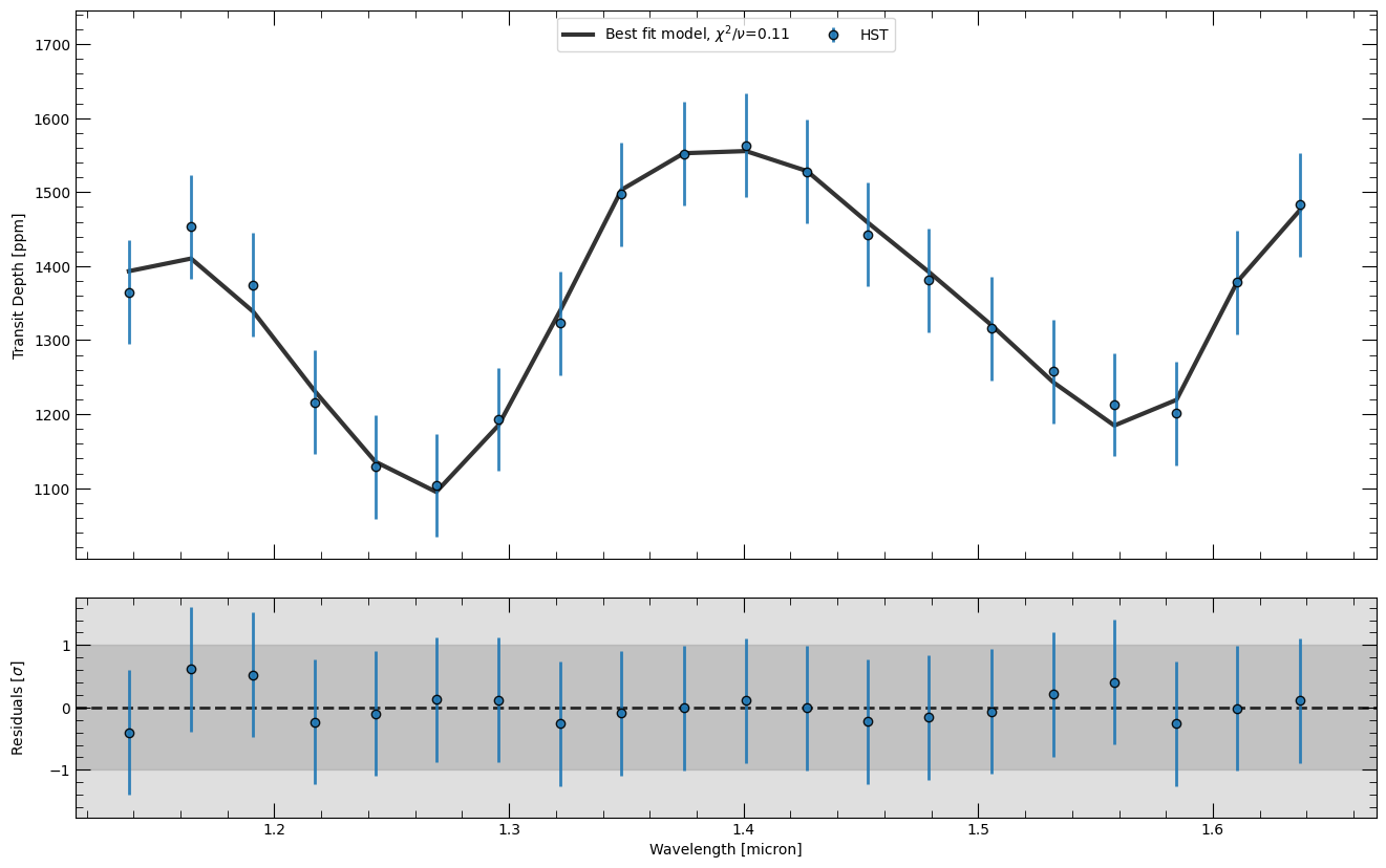
Best Fit Spectrum#
Here we will plot the best fit spectrum, together with the data used in the retrieval and the residuals between the two. Using the mode parameter, it is also possible to plot the spectrum using the 'median' fit instead of the maximum likelihood sample. The chi squared value presented in the figure is the reduced chi square, that is the chi square divided by the degrees of freedom (number of data points - number of parameters).
[10]:
# Plotting the best fit spectrum
# This will generate a few warnings, but it's fine.
fig, ax, ax_r = retrieval.plot_spectra(samples_use, parameters_read, refresh=True, mode="bestfit")
Not in evaluate mode. Changing run mode to evaluate.

Plotting Best-fit spectrum
Best fit likelihood = 172.31
Loading Radtrans opacities...
 Loading line opacities of species '1H2-16O__POKAZATEL.R120' from file '/Users/nasedkin/python-packages/petitRADTRANS/input_data/opacities/lines/correlated_k/H2O/1H2-16O/1H2-16O__POKAZATEL.R120_0.3-50mu.ktable.petitRADTRANS.h5'... Done.
 Loading line opacities of species '12C-1H4__HITEMP.R120' from file '/Users/nasedkin/python-packages/petitRADTRANS/input_data/opacities/lines/correlated_k/CH4/12C-1H4/12C-1H4__HITEMP.R120_0.1-250mu.ktable.petitRADTRANS.h5'... Done.
 Loading line opacities of species '12C-16O2__UCL-4000.R120' from file '/Users/nasedkin/python-packages/petitRADTRANS/input_data/opacities/lines/correlated_k/CO2/12C-16O2/12C-16O2__UCL-4000.R120_0.3-50mu.ktable.petitRADTRANS.h5'... Done.
 Loading line opacities of species 'C-O-NatAbund__HITEMP.R120' from file '/Users/nasedkin/python-packages/petitRADTRANS/input_data/opacities/lines/correlated_k/CO/C-O-NatAbund/C-O-NatAbund__HITEMP.R120_0.1-250mu.ktable.petitRADTRANS.h5'... Done.
 Successfully loaded all line opacities
 Loading CIA opacities for H2--H2 from file '/Users/nasedkin/python-packages/petitRADTRANS/input_data/opacities/continuum/collision_induced_absorptions/H2--H2/H2--H2-NatAbund/H2--H2-NatAbund__BoRi.R831_0.6-250mu.ciatable.petitRADTRANS.h5'... Done.
 Loading CIA opacities for H2--He from file '/Users/nasedkin/python-packages/petitRADTRANS/input_data/opacities/continuum/collision_induced_absorptions/H2--He/H2--He-NatAbund/H2--He-NatAbund__BoRi.DeltaWavenumber2_0.5-500mu.ciatable.petitRADTRANS.h5'... Done.
 Successfully loaded all CIA opacities
Successfully loaded all opacities
Best fit 𝛘^2 = 1.35
Best fit 𝛘^2/DoF = 0.11
/Users/nasedkin/python-packages/petitRADTRANS/petitRADTRANS/retrieval/plotting.py:1780: UserWarning: This figure includes Axes that are not compatible with tight_layout, so results might be incorrect.
  plt.tight_layout()
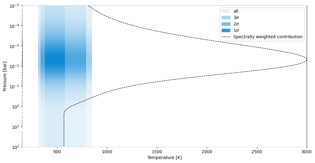
Pressure-Temperature profile#
Here we show the retrieved pressure-temperature profile throughout the atmosphere. The contours show the 1, 2 and 3 sigma confidence intervals in temperature around the median retrieved profile. If contribution=True, the opacity shading and dashed line show the region of the atmosphere that contributes to the observed spectrum, highlighting which part of the pressure profile is being probed.
[11]:
# Plotting the PT profile
fig, ax = retrieval.plot_pt(sample_dict, parameters_read, contribution=True)
INFO:arviz:Found 'auto' as default backend, checking available backends
INFO:arviz:Matplotlib is available, defining as default backend
INFO:arviz:arviz_base 1.1.0 available, exposing its functions as part of the `arviz` namespace
INFO:arviz:arviz_stats 1.1.0 available, exposing its functions as part of the `arviz` namespace
INFO:arviz:arviz_plots 1.1.0 available, exposing its functions as part of the `arviz` namespace
Plotting PT profiles
Best fit likelihood = 172.31
Loading best fit spectrum and contribution from file
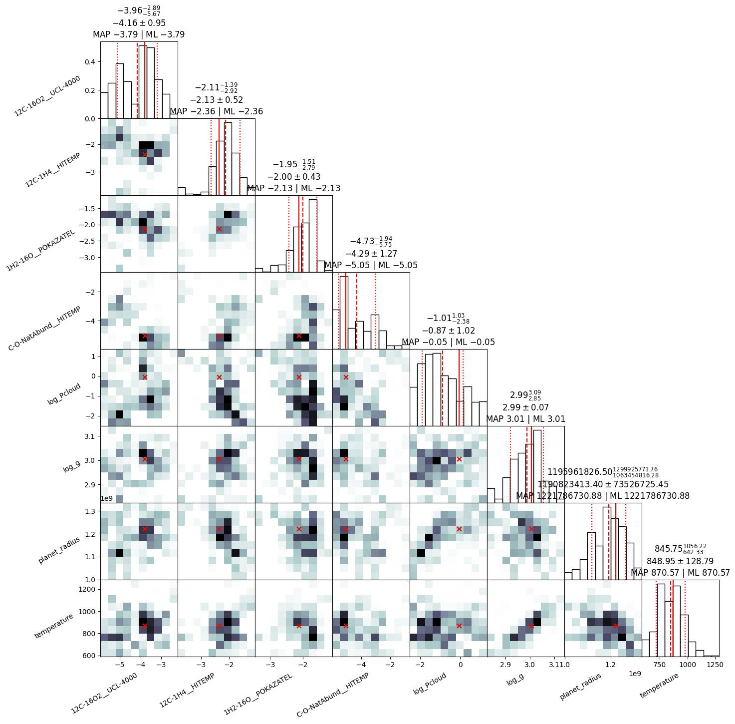
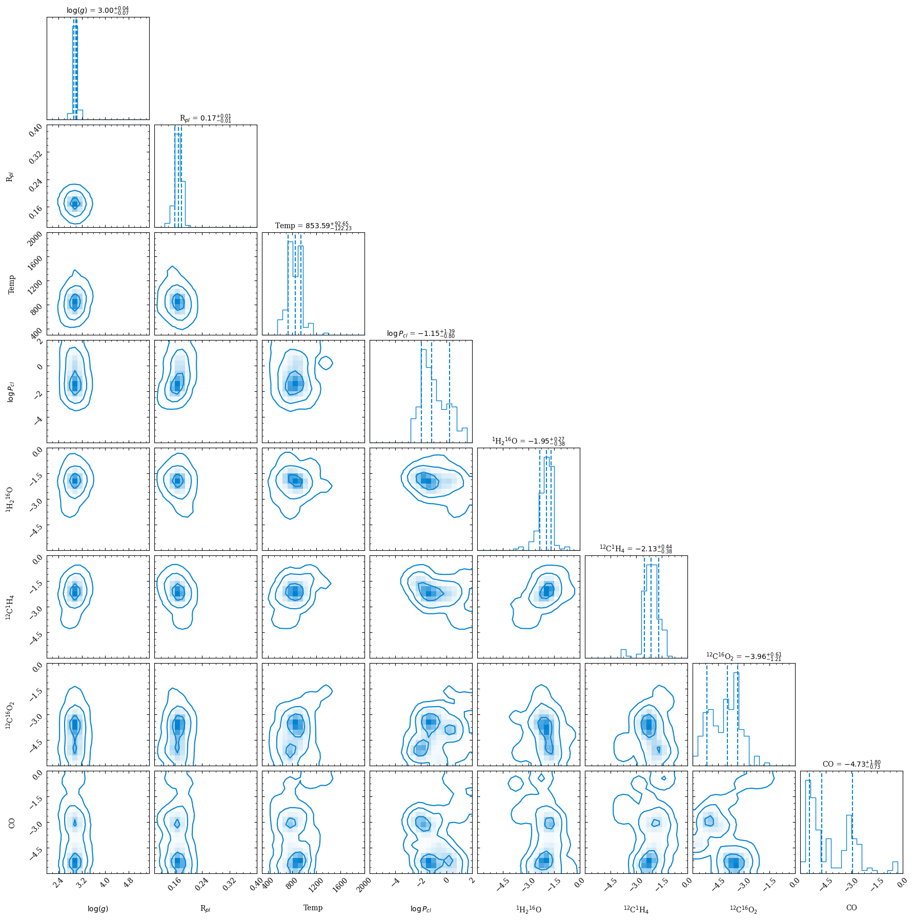
Corner plot#
Here we show the corner plot for the retrieval, which shows the marginal posterior probability distributions for each parameter (though it is also possibe to plot only a subset of the parameters). The corner plot produces 1, 2 and 3 sigma contours for the 2D plots, and highlights the 1 sigma confidence interval in the histograms for each parameter. Optional, there are several kwarg parameters that can be used to customise the plotting aesthetics.
[12]:
# Corner plot
# The corner plot produces 1,2 and 3 sigma contours for the 2D plots
retrieval.plot_corner(sample_dict, parameter_dict, parameters_read, title_kwargs={"fontsize": 10}, smooth=1)
Making corner plot
[12]:
Note that all plots, but also additional files (including the best-fit spectrum at high-resolution, so \(\lambda/\Delta\lambda=1000\), regardless of what your model resolution for the retrieval was), will also be put into the evaluate_hst_example_clear_spec folder.
Plot everything at once#
It is possible to plot every figures at once using the plot_all function. However, control on the figures is limited.
[13]:
retrieval.plot_all(contribution=True)
Best fit parameters
Best fit likelihood = 172.31
log_g 3.0052213165180444
planet_radius 1221786730.882757
temperature 870.5688700252059
log_Pcloud -0.045089298177894754
1H2-16O__POKAZATEL -2.128966371634534
12C-1H4__HITEMP -2.359282455090942
12C-16O2__UCL-4000 -3.785084699075592
C-O-NatAbund__HITEMP -5.053841809534646

Plotting Best-fit spectrum
Best fit likelihood = 172.31
Loading Radtrans opacities...
 Loading line opacities of species '1H2-16O__POKAZATEL.R120' from file '/Users/nasedkin/python-packages/petitRADTRANS/input_data/opacities/lines/correlated_k/H2O/1H2-16O/1H2-16O__POKAZATEL.R120_0.3-50mu.ktable.petitRADTRANS.h5'... Done.
 Loading line opacities of species '12C-1H4__HITEMP.R120' from file '/Users/nasedkin/python-packages/petitRADTRANS/input_data/opacities/lines/correlated_k/CH4/12C-1H4/12C-1H4__HITEMP.R120_0.1-250mu.ktable.petitRADTRANS.h5'... Done.
 Loading line opacities of species '12C-16O2__UCL-4000.R120' from file '/Users/nasedkin/python-packages/petitRADTRANS/input_data/opacities/lines/correlated_k/CO2/12C-16O2/12C-16O2__UCL-4000.R120_0.3-50mu.ktable.petitRADTRANS.h5'... Done.
 Loading line opacities of species 'C-O-NatAbund__HITEMP.R120' from file '/Users/nasedkin/python-packages/petitRADTRANS/input_data/opacities/lines/correlated_k/CO/C-O-NatAbund/C-O-NatAbund__HITEMP.R120_0.1-250mu.ktable.petitRADTRANS.h5'... Done.
 Successfully loaded all line opacities
 Loading CIA opacities for H2--H2 from file '/Users/nasedkin/python-packages/petitRADTRANS/input_data/opacities/continuum/collision_induced_absorptions/H2--H2/H2--H2-NatAbund/H2--H2-NatAbund__BoRi.R831_0.6-250mu.ciatable.petitRADTRANS.h5'... Done.
 Loading CIA opacities for H2--He from file '/Users/nasedkin/python-packages/petitRADTRANS/input_data/opacities/continuum/collision_induced_absorptions/H2--He/H2--He-NatAbund/H2--He-NatAbund__BoRi.DeltaWavenumber2_0.5-500mu.ciatable.petitRADTRANS.h5'... Done.
 Successfully loaded all CIA opacities
Successfully loaded all opacities
Best fit 𝛘^2 = 1.35
Best fit 𝛘^2/DoF = 0.11
/Users/nasedkin/python-packages/petitRADTRANS/petitRADTRANS/retrieval/plotting.py:1780: UserWarning: This figure includes Axes that are not compatible with tight_layout, so results might be incorrect.
  plt.tight_layout()
Plotting PT profiles
Best fit likelihood = 172.31
Loading best fit spectrum and contribution from file

Making corner plot

Plotting Best-fit contribution function
Best fit likelihood = 172.31
Loading best fit spectrum and contribution from file

Plotting Abundances profiles
Best fit likelihood = 172.31
Loading best fit spectrum and contribution from file
Finished generating all plots!
Contact
If you need any additional help, don’t hesitate to contact Evert Nasedkin.