Retrievals: Using the Model Functions

Written by Evert Nasedkin.

Please cite pRT’s retrieval package (Nasedkin et al. 2024) in addition to pRT (Mollière et al. 2019) if you make use of the retrieval package for your work.

This notebook is the update to the legacy models tutorial. It shows how to call the new model function interface directly — outside of a full retrieval loop — to compute spectra and temperature profiles.

The new interface differs from the legacy one in two key ways:

• The first argument is a ModelContext (containing the Radtrans object and evaluation flags) instead of the bare Radtrans object.

• The second argument is a PhysicalParams mapping (values accessed directly with params['key']) instead of a dict of Parameter objects (accessed with params['key'].value).

This interface is required when using the JAXNS sampler, and is also the recommended path for new custom models because it is fully JAX-traceable.

As with retrieval_models.ipynb, the cells below calculate models in isolation. In a real retrieval you would register the same function via add_data(..., model_generating_function=...) and the RetrievalConfig / Retrieval machinery handles everything else.

import jax
jax.config.update("jax_enable_x64", True)
import jax.numpy as jnp

import matplotlib.pyplot as plt

import petitRADTRANS as prt
from petitRADTRANS.retrieval.runtime import ModelInputs, ModelResult
from petitRADTRANS.retrieval.models import (
    molliere_2020_emission,
    guillot_emission,
    guillot_relative_emission,
    gradient_profile_emission,
    guillot_transmission,
    isothermal_transmission,
    calculate_transmission_spectrum_runtime,
)
from petitRADTRANS.retrieval.runtime import ModelContext, PhysicalParams
from petitRADTRANS.plotlib.style import set_petitradtrans_plot_style
from petitRADTRANS import physical_constants as cst


set_petitradtrans_plot_style()
print(f"JAX devices: {jax.devices()}")

Using pRT Plotting style!
JAX devices: [CpuDevice(id=0)]

The ModelContext and PhysicalParams objects

Every model function has the signature:

def my_model(model_context: ModelContext, physical_params: PhysicalParams, pt_plot_mode: bool = False) -> ModelResult:
    ...

• ``ModelContext`` is a frozen dataclass that carries the Radtrans object plus evaluation flags such as return_contribution, adaptive_mesh_refinement, etc.

• ``PhysicalParams`` is a JAX-pytree-compatible mapping of parameter name → scalar value. Unlike the legacy Parameter dict, you access values directly: physical_params['log_g'] rather than parameters['log_g'].value.

• The return value is a ``ModelResult`` with fields wavelengths, spectrum, pressures, temperatures, and auxiliary_outputs.

Both objects are constructed from plain Python dicts, as shown in the examples below.

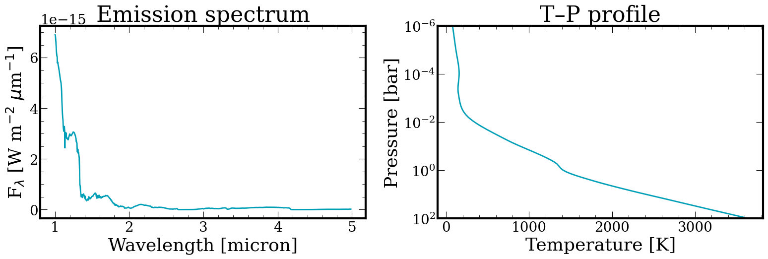
Emission spectrum: spline_eddington_adiabatic_emission

We set up a Radtrans object and compute a disequilibrium-chemistry emission spectrum for an HR 8799-like planet using the Mollière 2020 temperature profile.

The same set-up can be used for any of the runtime-native emission functions; just swap the function name and adjust the parameter dictionary accordingly.

line_species = (
    "H2O__POKAZATEL.R300",
    "CO-NatAbund.R300",
    "CH4.R300",
    "CO2.R300",
    "H2S.R300",
    "NH3.R300",
)

rayleigh_species = ("H2", "He")
continuum_opacities = ("H2--H2", "H2--He")
pressures = jnp.logspace(-6, 2, 100)

atmosphere_emission = prt.radtrans.Radtrans(
    pressures=pressures,
    line_species=line_species,
    rayleigh_species=rayleigh_species,
    gas_continuum_contributors=continuum_opacities,
    cloud_species=(),
    wavelength_boundaries=(1, 5),
)

Loading Radtrans opacities...
 Loading line opacities of species 'H2O__POKAZATEL.R300' from file '/Users/nasedkin/python-packages/petitRADTRANS/input_data/opacities/lines/correlated_k/H2O/1H2-16O/1H2-16O__POKAZATEL.R300_0.3-50mu.ktable.petitRADTRANS.h5'... Done.
 Loading line opacities of species 'CO-NatAbund.R300' from file '/Users/nasedkin/python-packages/petitRADTRANS/input_data/opacities/lines/correlated_k/CO/C-O-NatAbund/C-O-NatAbund__HITEMP.R300_0.1-250mu.ktable.petitRADTRANS.h5'... Done.
 Loading line opacities of species 'CH4.R300' from file '/Users/nasedkin/python-packages/petitRADTRANS/input_data/opacities/lines/correlated_k/CH4/12C-1H4/12C-1H4__YT34to10.R300_0.3-50mu.ktable.petitRADTRANS.h5'... Done.
 Loading line opacities of species 'CO2.R300' from file '/Users/nasedkin/python-packages/petitRADTRANS/input_data/opacities/lines/correlated_k/CO2/12C-16O2/12C-16O2__UCL-4000.R300_0.3-50mu.ktable.petitRADTRANS.h5'... Done.
 Loading line opacities of species 'H2S.R300' from file '/Users/nasedkin/python-packages/petitRADTRANS/input_data/opacities/lines/correlated_k/H2S/1H2-32S/1H2-32S__AYT2.R300_0.3-50mu.ktable.petitRADTRANS.h5'... Done.
 Loading line opacities of species 'NH3.R300' from file '/Users/nasedkin/python-packages/petitRADTRANS/input_data/opacities/lines/correlated_k/NH3/14N-1H3/14N-1H3__CoYuTe.R300_0.3-50mu.ktable.petitRADTRANS.h5'... Done.
 Successfully loaded all line opacities
 Loading CIA opacities for H2--H2 from file '/Users/nasedkin/python-packages/petitRADTRANS/input_data/opacities/continuum/collision_induced_absorptions/H2--H2/H2--H2-NatAbund/H2--H2-NatAbund__BoRi.R831_0.6-250mu.ciatable.petitRADTRANS.h5'... Done.
 Loading CIA opacities for H2--He from file '/Users/nasedkin/python-packages/petitRADTRANS/input_data/opacities/continuum/collision_induced_absorptions/H2--He/H2--He-NatAbund/H2--He-NatAbund__BoRi.DeltaWavenumber2_0.5-500mu.ciatable.petitRADTRANS.h5'... Done.
 Successfully loaded all CIA opacities
Successfully loaded all opacities

Building ModelContext and PhysicalParams

ModelContext accepts return_contribution=True to request the emission contribution function as an auxiliary output.

PhysicalParams.from_mapping() builds the parameter object from a plain dict. Values are accessed directly (no .value attribute).

# Build the ModelContext — holds the Radtrans object and evaluation flags.
emission_context = ModelContext(
    name="hr8799_emission",
    mode="evaluate",
    radtrans=atmosphere_emission,
    adaptive_mesh_refinement=False,
    return_contribution=False,
)

# Build PhysicalParams from a plain dict.
# Values are plain scalars (or JAX arrays) — no Parameter wrappers needed.
# We use the from_mapping method instead of the standard constructure so
# that we can have arbitrary parameter names for the model functions.
emission_params = PhysicalParams.from_mapping(
    {
        # System
        "distance_to_system": 41.3 * cst.pc,
        # Planet — two of (log_g, planet_radius, mass)
        "mass": 5.0 * cst.m_jup,
        "planet_radius": 1.0 * cst.r_jup_mean,
        # Mollière 2020 temperature profile
        "T_int": 1500.0,
        "T3": 0.8,
        "T2": 0.4,
        "T1": 0.5,
        "log_delta": 0.65,
        "alpha": 1.70,
        # Equilibrium chemistry
        "Fe/H": 1.0,
        "C/O": 0.7,
        "log_pquench": 2.5,
    }
)

Calling the model

The return value is a ModelResult. Use result.wavelengths and result.spectrum to get the spectrum, and result.pressures / result.temperatures when pt_plot_mode=True.

# Compute the emission spectrum
result = molliere_2020_emission(emission_context, emission_params, pt_plot_mode=False)
wavelengths = result.wavelengths
spectrum = result.spectrum

# Compute the T-P profile
pt_result = molliere_2020_emission(emission_context, emission_params, pt_plot_mode=True)
p_profile = pt_result.pressures
t_profile = pt_result.temperatures

Loading chemical equilibrium chemistry table from file '/Users/nasedkin/python-packages/petitRADTRANS/input_data/pre_calculated_chemistry/equilibrium_chemistry/equilibrium_chemistry.chemtable.petitRADTRANS.h5'... Done.

fig, axes = plt.subplots(1, 2, figsize=(16, 6))

axes[0].plot(wavelengths, spectrum, linewidth=2)
axes[0].set_xlabel("Wavelength [micron]")
axes[0].set_ylabel(r"F$_{\lambda}$ [W m$^{-2}$ $\mu$m$^{-1}$]")
axes[0].set_title("Emission spectrum")

axes[1].plot(t_profile, p_profile, linewidth=2)
axes[1].set_xlabel("Temperature [K]")
axes[1].set_ylabel("Pressure [bar]")
axes[1].set_ylim(1e2, 1e-6)
axes[1].set_yscale("log")
axes[1].set_title("T–P profile")

fig.tight_layout()

Other emission models

Swapping to a different built-in model requires only two changes: the function name and the parameter dictionary.

Guillot emission

Replace T1/T2/T3/log_delta/alpha with T_equ, gamma, and log_kappa_IR.

guillot_context = ModelContext(
    name="guillot_emission_demo",
    mode="evaluate",
    radtrans=atmosphere_emission,
    adaptive_mesh_refinement=False,
)

guillot_params = PhysicalParams.from_mapping(
    {
        "distance_to_system": 41.3 * cst.pc,
        "mass": 5.0 * cst.m_jup,
        "planet_radius": 1.0 * cst.r_jup_mean,
        # Guillot temperature profile
        "T_int": 700.0,
        "T_equ": 1300.0,
        "gamma": 0.4,
        "log_kappa_IR": -1.5,
        # Equilibrium chemistry
        "Fe/H": 1.0,
        "C/O": 0.7,
        "log_pquench": 2.5,
    }
)

guillot_result = guillot_emission(guillot_context, guillot_params)
print(f"Computed {guillot_result.wavelengths.shape[0]} wavelength points.")

Computed 482 wavelength points.

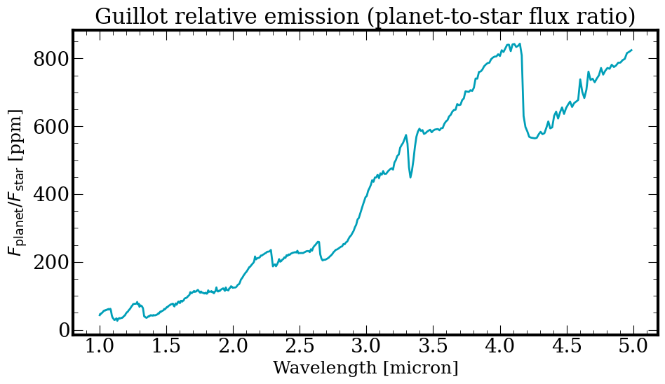
Guillot relative emission (planet-to-star flux ratio)

guillot_relative_emission uses exactly the same Guillot temperature profile and atmospheric chemistry as guillot_emission, but normalises the resulting planet flux by a PHOENIX stellar spectrum rebinned to the same wavelength grid. The returned spectrum is the dimensionless ratio \(F_\mathrm{planet} / F_\mathrm{star}\), suitable for secondary-eclipse or direct-imaging contrast retrieval.

Two extra parameters are required compared to guillot_emission:

Parameter	Description
star_effective_temperature	Stellar effective temperature in K
stellar_radius	Stellar radius in cm (optional — PHOENIX default used if omitted)

The example below reuses the same Radtrans object as the previous Guillot section and adds a Sun-like host star.

# Reuse the same Radtrans object as above (atmosphere_emission).
rel_emission_context = ModelContext(
    name="guillot_relative_emission_demo",
    mode="evaluate",
    radtrans=atmosphere_emission,
    adaptive_mesh_refinement=False,
)

# Parameters for the planet (same Guillot profile as the guillot_emission example
# above) plus the two new stellar parameters.
rel_emission_params = PhysicalParams.from_mapping(
    {
        # System
        "distance_to_system": 41.3 * cst.pc,
        # Planet — two of (log_g, planet_radius, mass)
        "mass": 5.0 * cst.m_jup,
        "planet_radius": 1.0 * cst.r_jup_mean,
        # Guillot temperature profile
        "T_int": 700.0,
        "T_equ": 1300.0,
        "gamma": 0.4,
        "log_kappa_IR": -1.5,
        # Equilibrium chemistry
        "Fe/H": 1.0,
        "C/O": 0.7,
        "log_pquench": 2.5,
        # Host star (Sun-like)
        "star_effective_temperature": 5778.0,  # K
        "stellar_radius": cst.r_sun,  # cm
    }
)

# Compute the planet-to-star flux ratio.
rel_result = guillot_relative_emission(rel_emission_context, rel_emission_params)
print(
    f"Computed {rel_result.wavelengths.shape[0]} wavelength points.  "
    f"Peak contrast: {float(rel_result.spectrum.max()):.2e}"
)

Loading PHOENIX star table in file '/Users/nasedkin/python-packages/petitRADTRANS/input_data/stellar_spectra/phoenix/phoenix.startable.petitRADTRANS.h5'... Done.
Computed 482 wavelength points.  Peak contrast: 8.43e-04

fig, ax = plt.subplots(figsize=(10, 6))

ax.plot(rel_result.wavelengths, rel_result.spectrum * 1e6, linewidth=2)
ax.set_xlabel("Wavelength [micron]", fontsize=18)
ax.set_ylabel(r"$F_\mathrm{planet} / F_\mathrm{star}$ [ppm]", fontsize=18)
ax.set_title("Guillot relative emission (planet-to-star flux ratio)", fontsize=22)

fig.tight_layout()

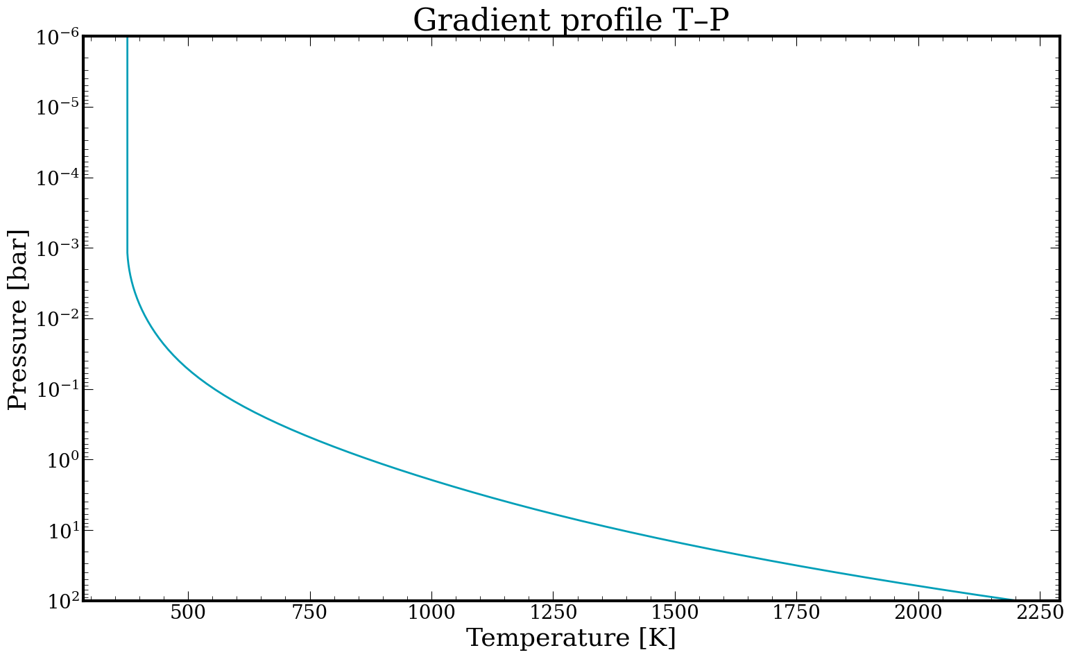
Gradient profile (dT/d log P) emission

This model is described in Zhang et al. (2023). The parameters are:

• N_layers: number of pressure layers.

• T_bottom: temperature at the deepest pressure level.

• PTslope_{i}: dT/d(log P) for each layer, from deep (i=1) to shallow (i=N_layers).

n_layers = 5

gradient_context = ModelContext(
    name="gradient_emission_demo",
    mode="evaluate",
    radtrans=atmosphere_emission,
    adaptive_mesh_refinement=False,
)

gradient_params = PhysicalParams.from_mapping(
    {
        "distance_to_system": 41.3 * cst.pc,
        "mass": 5.0 * cst.m_jup,
        "planet_radius": 1.0 * cst.r_jup_mean,
        # Gradient profile
        "N_layers": n_layers,
        "top_of_atmosphere_pressure": -3,
        "bottom_of_atmosphere_pressure": 2,
        "T_bottom": 2200.0,
        "PTslope_1": 0.2,
        "PTslope_2": 0.2,
        "PTslope_3": 0.2,
        "PTslope_4": 0.1,
        "PTslope_5": 0.0,
        # Equilibrium chemistry
        "Fe/H": 0.5,
        "C/O": 0.55,
        "log_pquench": 1,
    }
)

gradient_pt = gradient_profile_emission(gradient_context, gradient_params, pt_plot_mode=True)

fig, ax = plt.subplots()
ax.plot(gradient_pt.temperatures, gradient_pt.pressures, linewidth=2)
ax.set_xlabel("Temperature [K]")
ax.set_ylabel("Pressure [bar]")
ax.set_ylim(1e2, 1e-6)
ax.set_yscale("log")
ax.set_title("Gradient profile T–P")
fig.tight_layout()

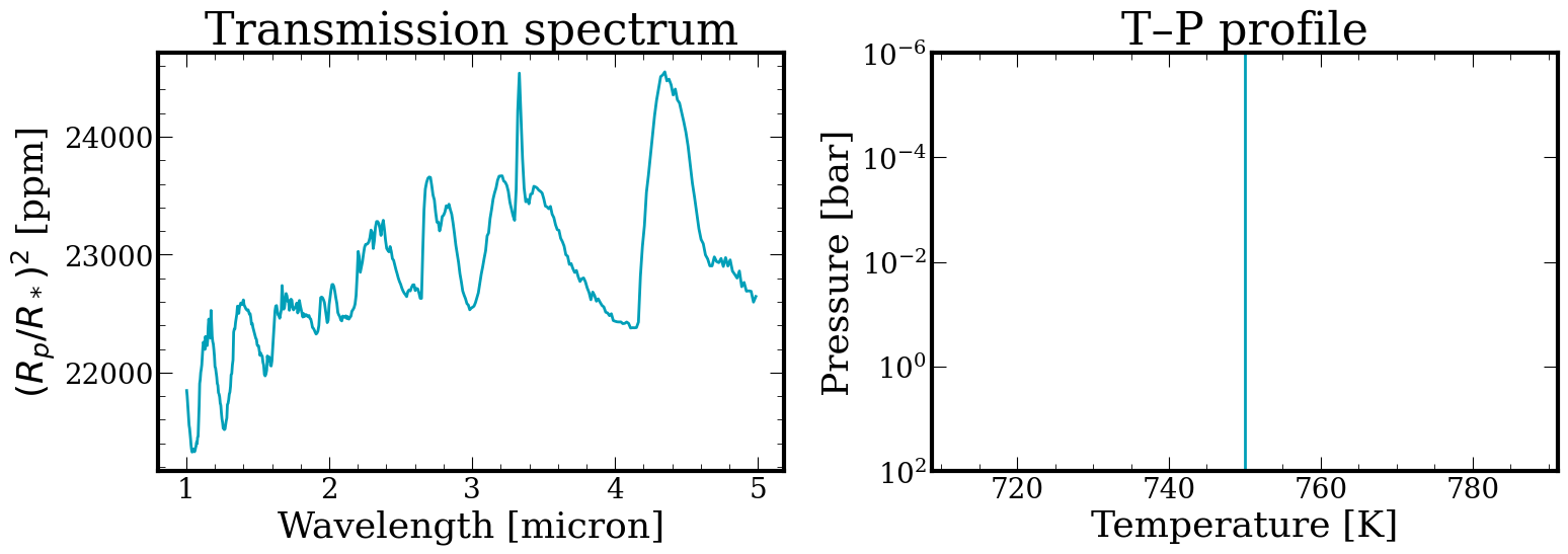
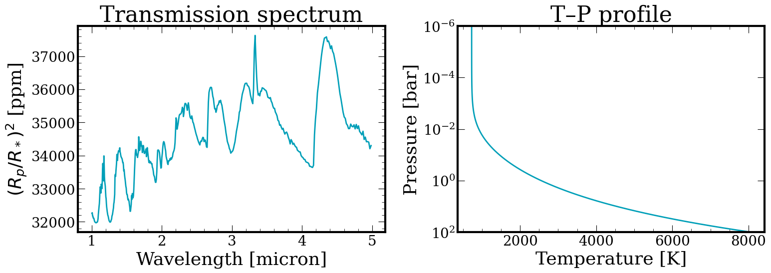
Transmission spectrum: guillot_transmission

For transmission models the required planet/star parameters are slightly different: stellar_radius must be provided (used to normalise the transit depth), and distance_to_system is not needed. A reference_pressure sets the pressure level at which planet_radius is defined (default: 100 bar).

We set up a WASP-39b-like planet.

atmosphere_transmission = prt.radtrans.Radtrans(
    pressures=pressures,
    line_species=(
        "H2O__POKAZATEL.R300",
        "CO-NatAbund.R300",
        "CH4.R300",
        "CO2.R300",
    ),
    rayleigh_species=("H2", "He"),
    gas_continuum_contributors=("H2--H2", "H2--He"),
    cloud_species=(),
    wavelength_boundaries=(1, 5),
)

Loading Radtrans opacities...
 Loading line opacities of species 'H2O__POKAZATEL.R300' from file '/Users/nasedkin/python-packages/petitRADTRANS/input_data/opacities/lines/correlated_k/H2O/1H2-16O/1H2-16O__POKAZATEL.R300_0.3-50mu.ktable.petitRADTRANS.h5'... Done.
 Loading line opacities of species 'CO-NatAbund.R300' from file '/Users/nasedkin/python-packages/petitRADTRANS/input_data/opacities/lines/correlated_k/CO/C-O-NatAbund/C-O-NatAbund__HITEMP.R300_0.1-250mu.ktable.petitRADTRANS.h5'... Done.
 Loading line opacities of species 'CH4.R300' from file '/Users/nasedkin/python-packages/petitRADTRANS/input_data/opacities/lines/correlated_k/CH4/12C-1H4/12C-1H4__YT34to10.R300_0.3-50mu.ktable.petitRADTRANS.h5'... Done.
 Loading line opacities of species 'CO2.R300' from file '/Users/nasedkin/python-packages/petitRADTRANS/input_data/opacities/lines/correlated_k/CO2/12C-16O2/12C-16O2__UCL-4000.R300_0.3-50mu.ktable.petitRADTRANS.h5'... Done.
 Successfully loaded all line opacities
 Loading CIA opacities for H2--H2 from file '/Users/nasedkin/python-packages/petitRADTRANS/input_data/opacities/continuum/collision_induced_absorptions/H2--H2/H2--H2-NatAbund/H2--H2-NatAbund__BoRi.R831_0.6-250mu.ciatable.petitRADTRANS.h5'... Done.
 Loading CIA opacities for H2--He from file '/Users/nasedkin/python-packages/petitRADTRANS/input_data/opacities/continuum/collision_induced_absorptions/H2--He/H2--He-NatAbund/H2--He-NatAbund__BoRi.DeltaWavenumber2_0.5-500mu.ciatable.petitRADTRANS.h5'... Done.
 Successfully loaded all CIA opacities
Successfully loaded all opacities

transmission_context = ModelContext(
    name="wasp39_transmission",
    mode="evaluate",
    radtrans=atmosphere_transmission,
    adaptive_mesh_refinement=False,
    return_contribution=False,
)

transmission_params = PhysicalParams.from_mapping(
    {
        # Star
        "stellar_radius": 0.9324 * cst.r_sun,
        # Planet
        "planet_radius": 1.3 * cst.r_jup_mean,
        "log_g": 2.75,
        "reference_pressure": 100.0,
        # Isothermal temperature profile
        "temperature": 750.0,
        # Equilibrium chemistry
        "Fe/H": 1.0,
        "C/O": 0.55,
    }
)

trans_result = isothermal_transmission(transmission_context, transmission_params, pt_plot_mode=False)

trans_pt = isothermal_transmission(transmission_context, transmission_params, pt_plot_mode=True)

fig, axes = plt.subplots(1, 2, figsize=(16, 6))

axes[0].plot(trans_result.wavelengths, trans_result.spectrum * 1e6, linewidth=2)
axes[0].set_xlabel("Wavelength [micron]")
axes[0].set_ylabel(r"$(R_p/R_*)^2$ [ppm]")
axes[0].set_title("Transmission spectrum")

axes[1].plot(trans_pt.temperatures, trans_pt.pressures, linewidth=2)
axes[1].set_xlabel("Temperature [K]")
axes[1].set_ylabel("Pressure [bar]")
axes[1].set_ylim(1e2, 1e-6)
axes[1].set_yscale("log")
axes[1].set_title("T–P profile")

fig.tight_layout()

transmission_context = ModelContext(
    name="wasp39_transmission",
    mode="evaluate",
    radtrans=atmosphere_transmission,
    adaptive_mesh_refinement=False,
    return_contribution=False,
)

transmission_params = PhysicalParams.from_mapping(
    {
        # Star
        "stellar_radius": 0.9324 * cst.r_sun,
        # Planet
        "planet_radius": 1.3 * cst.r_jup_mean,
        "log_g": 2.75,
        "reference_pressure": 100.0,
        # Guillot temperature profile
        "T_int": 750.0,
        "T_equ": 600.0,
        "log_kappa_IR": -1.0,
        "gamma": 1.0,
        # Haze and gray cloud
        "log_Pcloud": -2.0,
        "power_law_opacity_350nm": 1e-4,
        "power_law_opacity_coefficient": -3,
        # Equilibrium chemistry
        "Fe/H": 1.0,
        "C/O": 0.55,
    }
)

trans_result = guillot_transmission(transmission_context, transmission_params, pt_plot_mode=False)

trans_pt = guillot_transmission(transmission_context, transmission_params, pt_plot_mode=True)

fig, axes = plt.subplots(1, 2, figsize=(16, 6))

axes[0].plot(trans_result.wavelengths, trans_result.spectrum * 1e6, linewidth=2)
axes[0].set_xlabel("Wavelength [micron]")
axes[0].set_ylabel(r"$(R_p/R_*)^2$ [ppm]")
axes[0].set_title("Transmission spectrum")

axes[1].plot(trans_pt.temperatures, trans_pt.pressures, linewidth=2)
axes[1].set_xlabel("Temperature [K]")
axes[1].set_ylabel("Pressure [bar]")
axes[1].set_ylim(1e2, 1e-6)
axes[1].set_yscale("log")
axes[1].set_title("T–P profile")

fig.tight_layout()

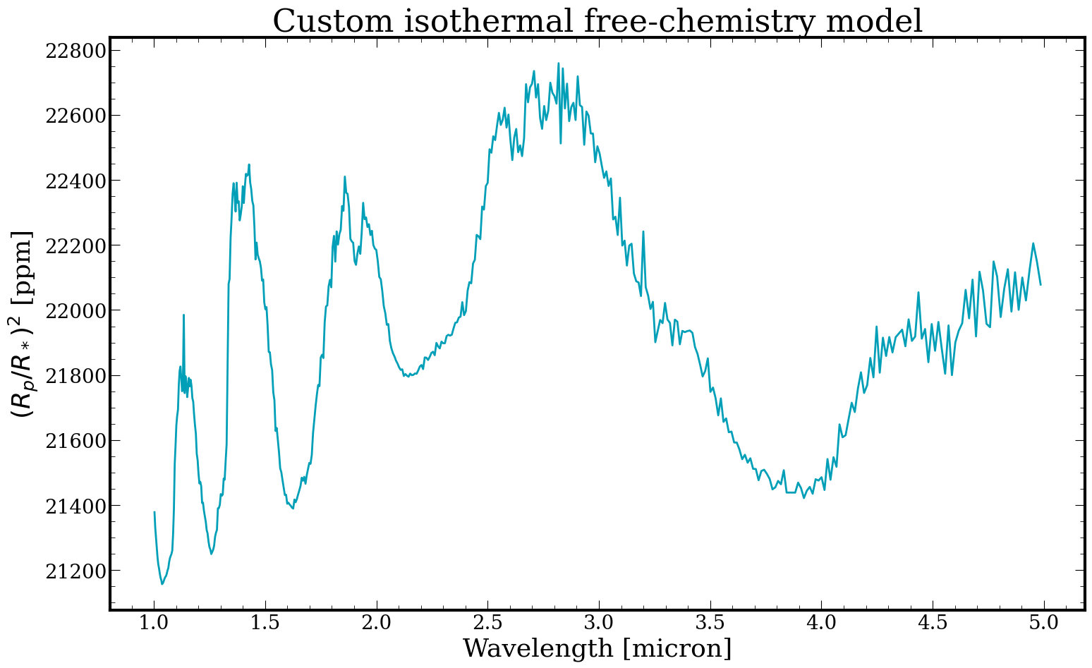
Writing a custom model

To write a custom model you only need to accept (model_context, physical_params, pt_plot_mode=False) and return a ModelResult. For simplicity, we delegate the actual radiative transfer to calculate_emission_spectrum_runtime or calculate_transmission_spectrum_runtime by constructing a ModelInputs container.

The example below adds a free-chemistry isothermal transmission model — the simplest possible case.

def custom_isothermal_free_chemistry_transmission(
    model_context: ModelContext,
    physical_params: PhysicalParams,
    pt_plot_mode: bool = False,
) -> ModelResult:
    """Isothermal transmission model with one free-chemistry species (H2O).

    Required parameters
    -------------------
    temperature         : isothermal temperature [K]
    log_g               : log10 surface gravity [cm/s^2]
    planet_radius       : planet radius [cm]
    stellar_radius      : stellar radius [cm]
    reference_pressure  : reference pressure for planet_radius [bar]
    log_H2O             : log10 H2O mass fraction
    log_Pcloud          : log10 gray cloud deck pressure [bar]
    """
    p = model_context.radtrans.pressures / 1e6  # bar
    temperatures = jnp.full_like(p, physical_params["temperature"])

    if pt_plot_mode:
        return ModelResult(kind="pt_profile", pressures=p, temperatures=temperatures)

    log_h2o = physical_params["log_H2O"]
    x_h2o = jnp.power(10.0, log_h2o)
    remainder = jnp.clip(1.0 - x_h2o, 1e-12, 1.0)

    # Build the mass fraction dict — keys must match line_species names
    abundances = {
        species: jnp.full_like(p, x_h2o) if "H2O" in species or "POKAZATEL" in species else jnp.full_like(p, 0.0)
        for species in model_context.radtrans.line_species
    }
    abundances["H2"] = jnp.full_like(p, 0.74 * remainder)
    abundances["He"] = jnp.full_like(p, 0.26 * remainder)

    model_inputs = ModelInputs(
        pressures=p,
        temperatures=temperatures,
        abundances=abundances,
        mean_molar_masses=jnp.full_like(p, 2.33),
        gravity=jnp.power(10.0, physical_params["log_g"]),
        planet_radius=physical_params["planet_radius"],
        stellar_radius=physical_params["stellar_radius"],
        reference_pressure=physical_params["reference_pressure"],
        opaque_cloud_top_pressure=jnp.power(10.0, physical_params["log_Pcloud"]),
    )

    return calculate_transmission_spectrum_runtime(model_context, model_inputs)

# Reuse the transmission Radtrans object from the previous section
custom_context = ModelContext(
    name="custom_isothermal",
    mode="evaluate",
    radtrans=atmosphere_transmission,
    adaptive_mesh_refinement=False,
)

custom_params = PhysicalParams.from_mapping(
    {
        "temperature": 900.0,
        "log_g": 2.75,
        "planet_radius": 1.3 * cst.r_jup_mean,
        "stellar_radius": 0.9324 * cst.r_sun,
        "reference_pressure": 100.0,
        "log_H2O": -3.0,
        "log_Pcloud": 0.0,
    }
)

custom_result = custom_isothermal_free_chemistry_transmission(custom_context, custom_params)

fig, ax = plt.subplots()
ax.plot(custom_result.wavelengths, custom_result.spectrum * 1e6, linewidth=2)
ax.set_xlabel("Wavelength [micron]")
ax.set_ylabel(r"$(R_p/R_*)^2$ [ppm]")
ax.set_title("Custom isothermal free-chemistry model")
fig.tight_layout()

Using the model in a retrieval

Once you have a model function it plugs straight into RetrievalConfig.add_data exactly like a legacy model:

from petitRADTRANS.retrieval import RetrievalConfig
from petitRADTRANS.retrieval.models import guillot_emission
import tensorflow_probability.substrates.jax as tfp

tfpd = tfp.distributions

retrieval_config = RetrievalConfig(
    retrieval_name='my_run',
    run_mode='retrieval',
    sampler_type='jaxns',
    pressures=pressures,
)

retrieval_config.add_parameter('log_g', is_free_parameter=True,
                               distribution=tfpd.Uniform(low=2.5, high=4.5))
# ... add remaining parameters ...

retrieval_config.add_data(
    name='my_data',
    path_to_observations='my_data.txt',
    model_generating_function=guillot_emission,  # or your custom function
    wavelength_boundaries=(1.0, 5.0),
    line_opacity_mode='c-k',
)

The retrieval runtime automatically detects the new model contract, ensuring that the forward model is fully differentiable for JAX-based samplers. See the JAX runtime emission tutorial for a complete end-to-end example including prior setup, runtime inspection, and running JAXNS.