Including clouds#

Let’s first make some useful imports.

[1]:

from jax import config
config.update("jax_enable_x64", True)

import jax.numpy as jnp
import matplotlib.pyplot as plt
import numpy as np

from petitRADTRANS.spectral_model import SpectralModel
from petitRADTRANS.radtrans import Radtrans
from petitRADTRANS.temperature_profiles import guillot_global_temperature_profile
from petitRADTRANS import physical_constants as cst

Let’s now instantiate a Radtrans object in the usual way, see “Getting Started”.

[2]:

atmosphere = Radtrans(
    pressures=jnp.logspace(-6, 2, 100),
    line_species=("H2O", "CO-NatAbund", "CH4", "CO2", "Na__NewAllard", "K__Allard"),
    rayleigh_species=("H2", "He"),
    gas_continuum_contributors=("H2--H2", "H2--He"),
    wavelength_boundaries=(0.3, 15),
    scattering_in_emission=False,
)

Loading Radtrans opacities...
Loading line opacities of species 'H2O' from file '/Users/nasedkin/python-packages/petitRADTRANS/input_data/opacities/lines/correlated_k/H2O/1H2-16O/1H2-16O__POKAZATEL.R1000_0.3-50mu.ktable.petitRADTRANS.h5'... Done.
Loading line opacities of species 'CO-NatAbund' from file '/Users/nasedkin/python-packages/petitRADTRANS/input_data/opacities/lines/correlated_k/CO/C-O-NatAbund/C-O-NatAbund__HITEMP.R1000_0.1-250mu.ktable.petitRADTRANS.h5'... Done.
Loading line opacities of species 'CH4' from file '/Users/nasedkin/python-packages/petitRADTRANS/input_data/opacities/lines/correlated_k/CH4/12C-1H4/12C-1H4__MM.R1000_0.3-50mu.ktable.petitRADTRANS.h5'... Done.
Loading line opacities of species 'CO2' from file '/Users/nasedkin/python-packages/petitRADTRANS/input_data/opacities/lines/correlated_k/CO2/12C-16O2/12C-16O2__UCL-4000.R1000_0.3-50mu.ktable.petitRADTRANS.h5'... Done.
Loading line opacities of species 'Na__NewAllard' from file '/Users/nasedkin/python-packages/petitRADTRANS/input_data/opacities/lines/correlated_k/Na/23Na/23Na__NewAllard.R1000_0.1-250mu.ktable.petitRADTRANS.h5'... Done.
Loading line opacities of species 'K__Allard' from file '/Users/nasedkin/python-packages/petitRADTRANS/input_data/opacities/lines/correlated_k/K/39K/39K__Allard.R1000_0.1-250mu.ktable.petitRADTRANS.h5'... Done.
Successfully loaded all line opacities
Loading CIA opacities for H2--H2 from file '/Users/nasedkin/python-packages/petitRADTRANS/input_data/opacities/continuum/collision_induced_absorptions/H2--H2/H2--H2-NatAbund/H2--H2-NatAbund__BoRi.R831_0.6-250mu.ciatable.petitRADTRANS.h5'... Done.
Loading CIA opacities for H2--He from file '/Users/nasedkin/python-packages/petitRADTRANS/input_data/opacities/continuum/collision_induced_absorptions/H2--He/H2--He-NatAbund/H2--He-NatAbund__BoRi.DeltaWavenumber2_0.5-500mu.ciatable.petitRADTRANS.h5'... Done.
Successfully loaded all CIA opacities
Successfully loaded all opacities

Next we set up the atmospheric parameters, with a parameter selection identical to the “Getting Started” case.

[16]:

planet_radius = 1.0 * cst.r_jup_mean
reference_gravity = 10**3.5
reference_pressure = 0.01

pressures = atmosphere.pressures * 1e-6  # cgs to bar
infrared_mean_opacity = 0.01
gamma = 0.4
intrinsic_temperature = 200
equilibrium_temperature = 1500

temperatures = guillot_global_temperature_profile(
    pressures=pressures,
    infrared_mean_opacity=infrared_mean_opacity,
    gamma=gamma,
    gravities=reference_gravity,
    intrinsic_temperature=intrinsic_temperature,
    equilibrium_temperature=equilibrium_temperature,
)

mass_fractions = {
    "H2": 0.74 * jnp.ones_like(temperatures),
    "He": 0.24 * jnp.ones_like(temperatures),
    "H2O": 1e-3 * jnp.ones_like(temperatures),
    "CO-NatAbund": 1e-2 * jnp.ones_like(temperatures),
    "CO2": 1e-5 * jnp.ones_like(temperatures),
    "CH4": 1e-6 * jnp.ones_like(temperatures),
    "Na__NewAllard": 1e-5 * jnp.ones_like(temperatures),
    "K__Allard": 1e-6 * jnp.ones_like(temperatures),
}

mean_molar_masses = 2.33 * jnp.ones_like(temperatures)

Units in petitRADTRANS: all units inside petitRADTRANS are in cgs. However, when interfacing with the code, you are expected to provide pressures in bars (more intuitive), and the mean molecular mass in atomic mass units. They will be converted to cgs units within the code.

Abundances in petitRADTRANS: remember that abundances in pRT are in units of mass fractions, not number fractions (aka volume mixing ratio, VMR). One can convert between mass fractions and VMRs by using \begin{equation} X_i = \frac{\mu_i}{\mu}n_i, \end{equation} where \(X_i\) is the mass fraction of species \(i\), \(\mu_i\) the mass of a single molecule/atom/ion/… of species \(i\), \(\mu\) is the atmospheric mean molar mass, and \(n_i\) is the VMR of species \(i\). This is implemented in petitRADTRANS.chemistry.utils.mass_fractions2volume_mixing_ratios() and petitRADTRANS.chemistry.utils.volume_mixing_ratios2mass_fractions().

Let’s now calculate a clear transmission spectrum, for reference. An example for the emission case is available in the “Emission spectra” section.

[17]:

wavelengths, transit_radii, _ = atmosphere.calculate_transit_radii(
    temperatures=temperatures,
    mass_fractions=mass_fractions,
    mean_molar_masses=mean_molar_masses,
    reference_gravity=reference_gravity,
    planet_radius=planet_radius,
    reference_pressure=reference_pressure,
)
transit_radii_clear = transit_radii / cst.r_jup_mean

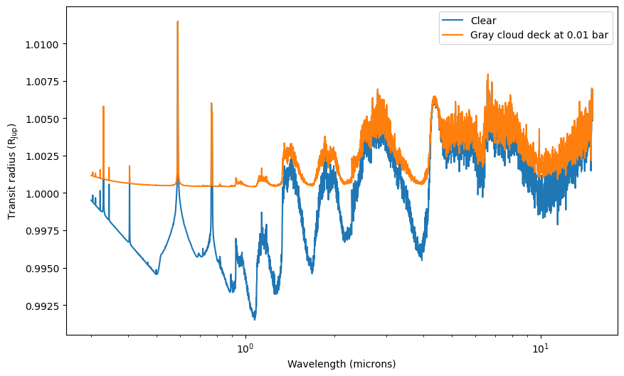
Gray cloud deck#

Now, let’s calculate cloudy spectra! The simplest way to add a cloud-like effect in petitRADTRANS is to add an opaque gray cloud deck. To do this, use the argument opaque_cloud_top_pressure (in bar).

Do not use this gray cloud deck implementation if you calculate pRT emission spectra in scattering mode. We increase the opacity to a very high value, \(10^{99}\) cm^2/g, at pressures > cloud top pressure. This can mess with the matrix inversion method used during the flux calculation. Please use the treatment explained here to define your own custom gray opacity in this case.

[5]:

# Opaque gray cloud deck at 0.01 bar
wavelengths, transit_radii_gray_cloud, _ = atmosphere.calculate_transit_radii(
    temperatures=temperatures,
    mass_fractions=mass_fractions,
    mean_molar_masses=mean_molar_masses,
    reference_gravity=reference_gravity,
    planet_radius=planet_radius,
    reference_pressure=reference_pressure,
    opaque_cloud_top_pressure=0.01,  # (bar)
)

[6]:

# Plot the spectra
fig, ax = plt.subplots(figsize=(10, 6))

ax.plot(wavelengths * 1e4, transit_radii_clear, label="Clear")
ax.plot(wavelengths * 1e4, transit_radii_gray_cloud / cst.r_jup_mean, label="Gray cloud deck at 0.01 bar")

ax.set_xscale("log")
ax.set_xlabel("Wavelength (microns)")
ax.set_ylabel(r"Transit radius ($\rm R_{Jup}$)")
ax.legend()

[6]:

<matplotlib.legend.Legend at 0x3217177d0>

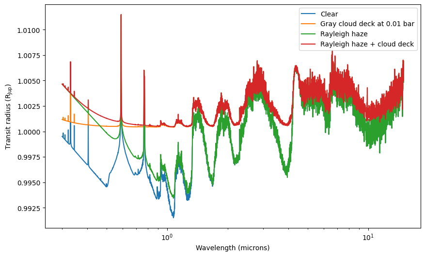
../../_images/content_notebooks_including_clouds_15_1.png

Scaled Rayleigh scattering#

It is also possible to mimick hazes effects by scaling the Rayleigh scattering opacities of the gas by a given factor, using the haze_factor argument.

[7]:

# Haze (10 x gas Rayleigh scattering)
wavelengths, transit_radii_hazy, _ = atmosphere.calculate_transit_radii(
    temperatures=temperatures,
    mass_fractions=mass_fractions,
    mean_molar_masses=mean_molar_masses,
    reference_gravity=reference_gravity,
    planet_radius=planet_radius,
    reference_pressure=reference_pressure,
    haze_factor=10.0,
)

This can be combined with the gray cloud deck.

Technically, any of the methods to include clouds presented here can be combined, although it does not necessarily makes sense to do so.

[8]:

# Haze + cloud deck
wavelengths, transit_radii_cloud_haze, _ = atmosphere.calculate_transit_radii(
    temperatures=temperatures,
    mass_fractions=mass_fractions,
    mean_molar_masses=mean_molar_masses,
    reference_gravity=reference_gravity,
    planet_radius=planet_radius,
    reference_pressure=reference_pressure,
    opaque_cloud_top_pressure=0.01,
    haze_factor=10.0,
)

[9]:

# Plot the spectra
fig, ax = plt.subplots(figsize=(10, 6))

ax.plot(wavelengths * 1e4, transit_radii_clear, label="Clear")
ax.plot(wavelengths * 1e4, transit_radii_gray_cloud / cst.r_jup_mean, label="Gray cloud deck at 0.01 bar")
ax.plot(wavelengths * 1e4, transit_radii_hazy / cst.r_jup_mean, label="Rayleigh haze")
ax.plot(wavelengths * 1e4, transit_radii_cloud_haze / cst.r_jup_mean, label="Rayleigh haze + cloud deck")

ax.set_xscale("log")
ax.set_xlabel("Wavelength (microns)")
ax.set_ylabel(r"Transit radius ($\rm R_{Jup}$)")
ax.legend()

[9]:

<matplotlib.legend.Legend at 0x167f971a0>

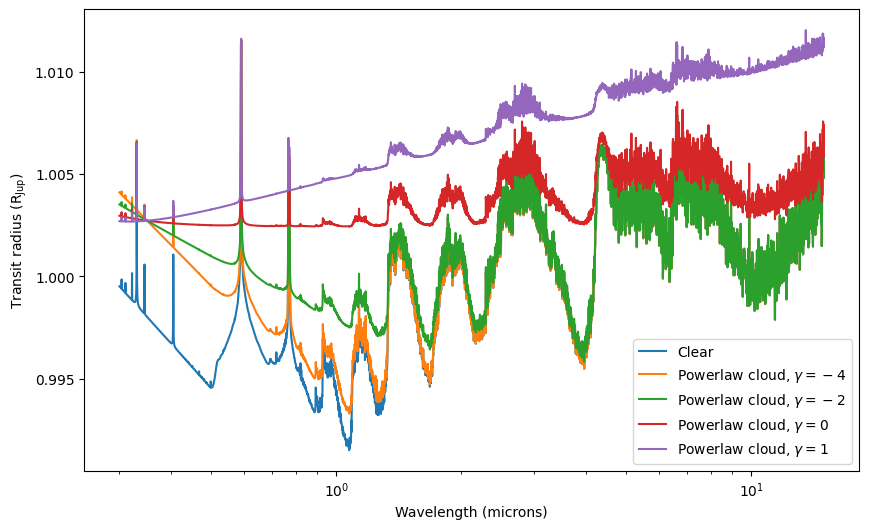
../../_images/content_notebooks_including_clouds_22_1.png

Powerlaw cloud models#

The next available mode is the so-called power law cloud. In this case the following opacity is added to the scattering cross-section: \begin{equation} \kappa = \kappa_0\left(\frac{\lambda}{\lambda_0}\right)^\gamma \end{equation} Where \(\kappa_0\) is the opacity at a given wavelength (here \(\lambda_0=0.35 \ {\rm \mu m}\)) in units of cm\(^2\)/g. The power law index \(\gamma\) fixes the wavelength dependence, Rayleigh-like scattering would be obtained for \(\gamma=-4\). Hence \(\kappa_0\) and \(\gamma\) are free parameters.

In petitRADTRANS, \(\kappa_0\) is set with the power_law_opacity_350nm argument, and \(\gamma\) by the power_law_opacity_coefficient argument.

Both power_law_opacity_350nm and power_law_opacity_coefficient must be set for the power law cloud to take effect.

We now calculate four power law cloudy models, with \(\kappa_0 = 0.01\) cm\(^2\)/g, and four different \(\gamma\) values.

First, \(\gamma = -4\) (Rayleigh-like):

[10]:

power_law_opacity_350nm = 0.01
power_law_opacity_coefficient = -4.0

wavelengths, transit_radii, _ = atmosphere.calculate_transit_radii(
    temperatures=temperatures,
    mass_fractions=mass_fractions,
    mean_molar_masses=mean_molar_masses,
    reference_gravity=reference_gravity,
    planet_radius=planet_radius,
    reference_pressure=reference_pressure,
    power_law_opacity_350nm=power_law_opacity_350nm,
    power_law_opacity_coefficient=power_law_opacity_coefficient,
)

transit_radii_gamma_m4 = transit_radii / cst.r_jup_mean

Second, \(\gamma = -2\) (weaker scattering power law):

[11]:

power_law_opacity_350nm = 0.01
power_law_opacity_coefficient = -2.0

wavelengths, transit_radii, _ = atmosphere.calculate_transit_radii(
    temperatures=temperatures,
    mass_fractions=mass_fractions,
    mean_molar_masses=mean_molar_masses,
    reference_gravity=reference_gravity,
    planet_radius=planet_radius,
    reference_pressure=reference_pressure,
    power_law_opacity_350nm=power_law_opacity_350nm,
    power_law_opacity_coefficient=power_law_opacity_coefficient,
)

transit_radii_gamma_m2 = transit_radii / cst.r_jup_mean

Third, \(\gamma = 0\) (flat opacity):

[12]:

power_law_opacity_350nm = 0.01
power_law_opacity_coefficient = 0.0

wavelengths, transit_radii, _ = atmosphere.calculate_transit_radii(
    temperatures=temperatures,
    mass_fractions=mass_fractions,
    mean_molar_masses=mean_molar_masses,
    reference_gravity=reference_gravity,
    planet_radius=planet_radius,
    reference_pressure=reference_pressure,
    power_law_opacity_350nm=power_law_opacity_350nm,
    power_law_opacity_coefficient=power_law_opacity_coefficient,
)

transit_radii_gamma0 = transit_radii / cst.r_jup_mean

Fourth, the exoctic case of, \(\gamma = 1\) (positive opacity slope):

[13]:

power_law_opacity_350nm = 0.01
power_law_opacity_coefficient = 1.0

wavelengths, transit_radii, _ = atmosphere.calculate_transit_radii(
    temperatures=temperatures,
    mass_fractions=mass_fractions,
    mean_molar_masses=mean_molar_masses,
    reference_gravity=reference_gravity,
    planet_radius=planet_radius,
    reference_pressure=reference_pressure,
    power_law_opacity_350nm=power_law_opacity_350nm,
    power_law_opacity_coefficient=power_law_opacity_coefficient,
)

transit_radii_gamma_p1 = transit_radii / cst.r_jup_mean

Let’s now make the plots.

[14]:

fig, ax = plt.subplots(figsize=(10, 6))

ax.plot(wavelengths * 1e4, transit_radii_clear, label="Clear")
ax.plot(wavelengths * 1e4, transit_radii_gamma_m4, label=r"Powerlaw cloud, $\gamma = -4$")
ax.plot(wavelengths * 1e4, transit_radii_gamma_m2, label=r"Powerlaw cloud, $\gamma = -2$")
ax.plot(wavelengths * 1e4, transit_radii_gamma0, label=r"Powerlaw cloud, $\gamma = 0$")
ax.plot(wavelengths * 1e4, transit_radii_gamma_p1, label=r"Powerlaw cloud, $\gamma = 1$")

ax.set_xscale("log")
ax.set_xlabel("Wavelength (microns)")
ax.set_ylabel(r"Transit radius ($\rm R_{Jup}$)")
ax.legend(loc="best")

[14]:

<matplotlib.legend.Legend at 0x13b207fb0>

../../_images/content_notebooks_including_clouds_35_1.png

Condensate clouds from real optical constants#

Let’s calculate some spectra using opacities derived from optical constants of various materials. In this example we will take forsterite, that is, \(\rm Mg_2SiO_4\). For the list of available cloud species see “Available opacity species”.

Choose your favorite particle setup: petitRADTRANS offers multiple opacity versions for every given condensate, assuming either spherical (Mie scattering) or irreagularly shaped (DHS method = distribution of hollow spheres) particles. Moreover, opacities assuming a crystalline and/or amorphous internal structure can be used, where available.

We set up the atmosphere like before, this time loading the opacity of solid (s), crystalline, irregularly shaped particles (DHS method). The mode identifier for the \(\rm Mg_2SiO_4\) opacity therefore is 'Mg2SiO4(s)_crystalline__DHS'. Note that for some species only crystalline or amorphous cross-sections are available.

But now, let’s start! We simply give one additional cloud_species list to the Radtrans object, containing the name of the opacity species we want to use.

[15]:

atmosphere = Radtrans(
    pressures=jnp.logspace(-6, 2, 100),
    line_species=("H2O", "CO-NatAbund", "CH4", "CO2", "Na__NewAllard", "K__Allard"),
    rayleigh_species=("H2", "He"),
    gas_continuum_contributors=("H2--H2", "H2--He"),
    cloud_species=("Mg2SiO4(s)_crystalline_000__DHS",),
    wavelength_boundaries=(0.3, 15),
)

Next we will setup the amtosphere, with a parameter selection almost identical to the “Getting Started” case. We also add the mass fraction of the cloud species we are interested in now.

[16]:

mass_fractions = {
    "H2": 0.74 * jnp.ones_like(temperatures),
    "He": 0.24 * jnp.ones_like(temperatures),
    "H2O": 1e-3 * jnp.ones_like(temperatures),
    "CO-NatAbund": 1e-2 * jnp.ones_like(temperatures),
    "CO2": 1e-5 * jnp.ones_like(temperatures),
    "CH4": 1e-6 * jnp.ones_like(temperatures),
    "Na__NewAllard": 1e-5 * jnp.ones_like(temperatures),
    "K__Allard": 1e-6 * jnp.ones_like(temperatures),
    "Mg2SiO4(s)_crystalline_000__DHS": 5e-6 * jnp.ones_like(temperatures),
}

Setting the cloud particles size#

We have to define a few additional parameters for the clouds, to start the calculation. Since we here assume a log-normal paricle size distribution, we give the mean particle size and width of the distribution:

[17]:

# Here the cloud particle mean radii are vertically constant, but they can vary with pressure as well

cloud_particle_mean_radii = {"Mg2SiO4(s)_crystalline_000__DHS": 5e-5 * jnp.ones_like(temperatures)}  # (cm) i.e. 0.5 um

# a value of 1.0 would be a delta function, so we assume a very narrow distribtion here
cloud_particle_radius_distribution_std = 1.05

Now, let’s calculate a clear and cloudy spectrum to compare:

[18]:

fig, ax = plt.subplots(figsize=(10, 6))


wavelengths, transit_radii, _ = atmosphere.calculate_transit_radii(
    temperatures=temperatures,
    mass_fractions=mass_fractions,
    mean_molar_masses=mean_molar_masses,
    reference_gravity=reference_gravity,
    planet_radius=planet_radius,
    reference_pressure=reference_pressure,
    cloud_particle_mean_radii=cloud_particle_mean_radii,
    cloud_particle_radius_distribution_std=cloud_particle_radius_distribution_std,
)

ax.plot(wavelengths, transit_radii / cst.r_jup_mean, label="cloudy", zorder=2)

mass_fractions["Mg2SiO4(s)_crystalline_000__DHS"] = jnp.zeros_like(temperatures)

wavelengths, transit_radii, _ = atmosphere.calculate_transit_radii(
    temperatures=temperatures,
    mass_fractions=mass_fractions,
    mean_molar_masses=mean_molar_masses,
    reference_gravity=reference_gravity,
    planet_radius=planet_radius,
    reference_pressure=reference_pressure,
    cloud_particle_mean_radii=cloud_particle_mean_radii,
    cloud_particle_radius_distribution_std=cloud_particle_radius_distribution_std,
)

ax.plot(wavelengths, transit_radii / cst.r_jup_mean, label="clear", zorder=1)
ax.set_xscale("log")
ax.set_xlabel("Wavelength (microns)")
ax.set_ylabel(r"Transit radius ($\rm R_{Jup}$)")
ax.legend(loc="best")

[18]:

<matplotlib.legend.Legend at 0x13e226ab0>

../../_images/content_notebooks_including_clouds_48_1.png

Here one sees that there is a lot of additional absorption in the optical and near-IR. Also note the silicate (Si-O stretching mode) becoming visible at 10 micron.

Calculating the cloud particles size#

Fixed settling parameter#

Below we will not predefine the particle size. Instead we will calculate it with the “Eddysed” approach presented in Ackerman & Marley (2001). For this, one specifies an eddy diffusion coefficient (\(K_{zz}\), with units of cm\(^2\)/s), which describes the strength of vertical atmospheric mixing. The cloud particle size is then controlled by \(K_{zz}\), and the unitless settling parameter \(f_{\rm sed}\), which expresses the particles’ mass averaged settling velocity, when compared to the local atmospheric mixing speed. Also, a width for the log-normal particle size distribution must be specified. Here we use an atmospheric structure almost identical to the one above, with the difference that we also add amorphous and spherical iron cloud particles ('Fe(s)_amorphous__Mie').

[2]:

atmosphere = Radtrans(
    pressures=jnp.logspace(-6, 2, 100),
    line_species=("H2O", "CO-NatAbund", "CH4", "CO2", "Na__NewAllard", "K__Allard"),
    rayleigh_species=("H2", "He"),
    gas_continuum_contributors=("H2--H2", "H2--He"),
    cloud_species=("Mg2SiO4(s)_crystalline_000__DHS", "Fe(s)_amorphous__Mie"),
    wavelength_boundaries=(0.3, 15),
    scattering_in_emission=False,
)

Here we define the eddy diffusion parameters. Below we use different \(f_{\rm sed}\) for the two different cloud species:

cloud_f_sed = {
    'Mg2SiO4(s)_crystalline__DHS': 2.0,
    'Fe(s)_amorphous__Mie': 3.0
}

If all the clouds should use the same \(f_{\rm sed}\) we can just set:

cloud_f_sed = 2.0

[4]:

eddy_diffusion_coefficients = jnp.ones_like(temperatures) * 10**7.5
cloud_f_sed = {"Mg2SiO4(s)_crystalline_000__DHS": 2.0, "Fe(s)_amorphous__Mie": 3.0}

# We still assume a log-normal particle size distribution:
cloud_particle_radius_distribution_std = 1.05

mass_fractions["Mg2SiO4(s)_crystalline_000__DHS"] = jnp.zeros_like(temperatures)
mass_fractions["Fe(s)_amorphous__Mie"] = jnp.zeros_like(temperatures)

Again, let’s calculate a clear and cloudy spectrum to compare:

[8]:

fig, ax = plt.subplots(figsize=(10, 6))

mass_fractions["Mg2SiO4(s)_crystalline_000__DHS"] = 5e-7 * jnp.ones_like(temperatures)
mass_fractions["Fe(s)_amorphous__Mie"] = 5e-7 * jnp.ones_like(temperatures)

wavelengths, transit_radii, additional_output = atmosphere.calculate_transit_radii(
    temperatures=temperatures,
    mass_fractions=mass_fractions,
    mean_molar_masses=mean_molar_masses,
    reference_gravity=reference_gravity,
    planet_radius=planet_radius,
    reference_pressure=reference_pressure,
    eddy_diffusion_coefficients=eddy_diffusion_coefficients,
    cloud_f_sed=cloud_f_sed,
    cloud_particle_radius_distribution_std=cloud_particle_radius_distribution_std,
)

ax.plot(wavelengths, transit_radii / cst.r_jup_mean, label="cloudy", zorder=2)

mass_fractions["Mg2SiO4(s)_crystalline_000__DHS"] = jnp.zeros_like(temperatures)
mass_fractions["Fe(s)_amorphous__Mie"] = jnp.zeros_like(temperatures)

wavelengths, transit_radii, _ = atmosphere.calculate_transit_radii(
    temperatures=temperatures,
    mass_fractions=mass_fractions,
    mean_molar_masses=mean_molar_masses,
    reference_gravity=reference_gravity,
    planet_radius=planet_radius,
    reference_pressure=reference_pressure,
    eddy_diffusion_coefficients=eddy_diffusion_coefficients,
    cloud_f_sed=cloud_f_sed,
    cloud_particle_radius_distribution_std=cloud_particle_radius_distribution_std,
)

ax.plot(wavelengths, transit_radii / cst.r_jup_mean, label="clear", zorder=1)

ax.set_xscale("log")
ax.set_xlabel("Wavelength (microns)")
ax.set_ylabel(r"Transit radius ($\rm R_{Jup}$)")
ax.legend(loc="best")

[8]:

<matplotlib.legend.Legend at 0x311706720>

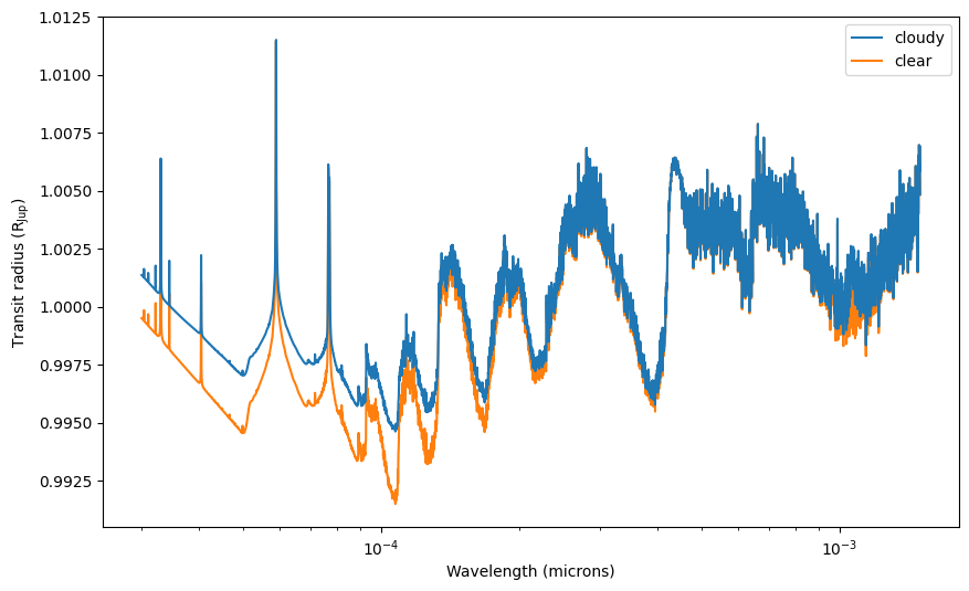
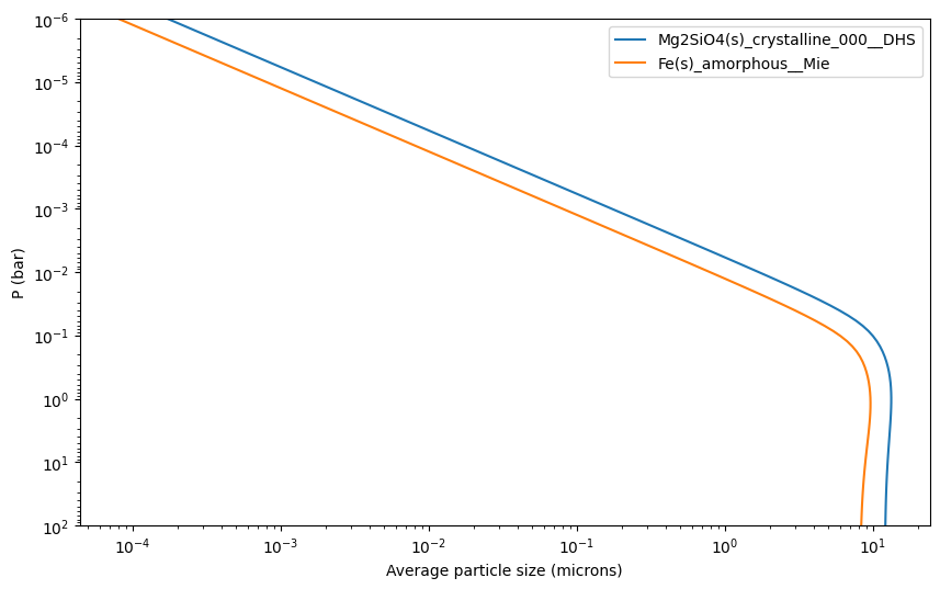
../../_images/content_notebooks_including_clouds_57_1.png

The resulting mean particle sizes can be accessed like this:

[9]:

fig, ax = plt.subplots(figsize=(10, 6))

ax.set_yscale("log")
ax.set_xscale("log")
ax.set_ylim([1e2, 1e-6])
ax.set_ylabel("P (bar)")
ax.set_xlabel("Average particle size (microns)")

for i_cloud in range(len(atmosphere.cloud_species)):
    ax.plot(
        additional_output["cloud_particle_mean_radii"][:, i_cloud] * 1e4,
        atmosphere.pressures * 1e-6,
        label=atmosphere.cloud_species[i_cloud],
    )

plt.legend()

[9]:

<matplotlib.legend.Legend at 0x3116fc860>

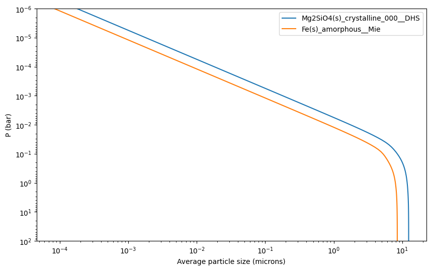
../../_images/content_notebooks_including_clouds_59_1.png

Particle sizes: the opacity of particles smaller than 1 nm and larger than 10 cm is set to zero.

Vertically variable settling parameter#

If you want you can also make cloud_f_sed vertically variable, here we set it vertically constant first and then scale it by scaling_factor_fsed.

[10]:

eddy_diffusion_coefficients = jnp.ones_like(temperatures) * 10**7.5
scaling_factor_fsed = jnp.ones_like(temperatures)
scaling_factor_fsed = jnp.where(atmosphere.pressures * 1e-6 < 1e-1, 0.1, scaling_factor_fsed)
cloud_f_sed = {
    "Mg2SiO4(s)_crystalline_000__DHS": 2.0 * jnp.ones_like(temperatures) * scaling_factor_fsed,
    "Fe(s)_amorphous__Mie": 3.0 * jnp.ones_like(temperatures) * scaling_factor_fsed,
}

# We still assume a log-normal particle size distribution:
cloud_particle_radius_distribution_std = 1.05

fig, ax = plt.subplots(figsize=(10, 6))

mass_fractions["Mg2SiO4(s)_crystalline_000__DHS"] = 5e-7 * jnp.ones_like(temperatures)
mass_fractions["Fe(s)_amorphous__Mie"] = 5e-7 * jnp.ones_like(temperatures)

wavelengths, transit_radii, additional_output = atmosphere.calculate_transit_radii(
    temperatures=temperatures,
    mass_fractions=mass_fractions,
    mean_molar_masses=mean_molar_masses,
    reference_gravity=reference_gravity,
    planet_radius=planet_radius,
    reference_pressure=reference_pressure,
    eddy_diffusion_coefficients=eddy_diffusion_coefficients,
    cloud_f_sed=cloud_f_sed,
    cloud_particle_radius_distribution_std=cloud_particle_radius_distribution_std,
)

ax.plot(wavelengths, transit_radii / cst.r_jup_mean, label="cloudy", zorder=2)

mass_fractions["Mg2SiO4(s)_crystalline_000__DHS"] = jnp.zeros_like(temperatures)
mass_fractions["Fe(s)_amorphous__Mie"] = jnp.zeros_like(temperatures)

wavelengths, transit_radii, _ = atmosphere.calculate_transit_radii(
    temperatures=temperatures,
    mass_fractions=mass_fractions,
    mean_molar_masses=mean_molar_masses,
    reference_gravity=reference_gravity,
    planet_radius=planet_radius,
    reference_pressure=reference_pressure,
    eddy_diffusion_coefficients=eddy_diffusion_coefficients,
    cloud_f_sed=cloud_f_sed,
    cloud_particle_radius_distribution_std=cloud_particle_radius_distribution_std,
)

ax.plot(wavelengths, transit_radii / cst.r_jup_mean, label="clear", zorder=1)

ax.set_xscale("log")
ax.set_xlabel("Wavelength (microns)")
ax.set_ylabel(r"Transit radius ($\rm R_{Jup}$)")
ax.legend(loc="best")

[10]:

<matplotlib.legend.Legend at 0x31145c440>

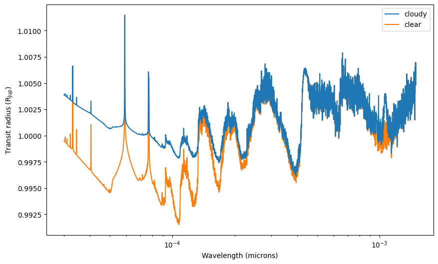
../../_images/content_notebooks_including_clouds_63_1.png

The resulting radii are smaller for pressures smaller than 0.1 bar.

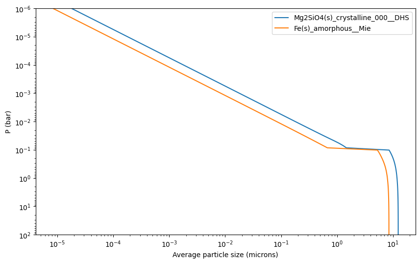
[11]:

fig, ax = plt.subplots(figsize=(10, 6))

ax.set_yscale("log")
ax.set_xscale("log")

ax.set_ylim([1e2, 1e-6])

ax.set_ylabel("P (bar)")
ax.set_xlabel("Average particle size (microns)")

for i_cloud in range(len(atmosphere.cloud_species)):
    ax.plot(
        additional_output["cloud_particle_mean_radii"][:, i_cloud] * 1e4,
        atmosphere.pressures * 1e-6,
        label=atmosphere.cloud_species[i_cloud],
    )

plt.legend()

[11]:

<matplotlib.legend.Legend at 0x31bbe5a30>

../../_images/content_notebooks_including_clouds_65_1.png

Hansen Distribution Clouds#

While the EddySed model used here typically uses a log-normal distribution for the cloud particle radii, it is also possible to use the Hansen (1971) distribution. To do this, you’ll need to set the cloud_particle_radius_distribution parameter in calculate_flux() or calculate_transit_radii() to 'hansen', and set the effective width of the distribution with the cloud_hansen_b parameter. Alternately, you can specify both the distribution width and center using the cloud_hansen_b and cloud_hansen_a arguments. Note that the value of cloud_hansen_b will be different from that of cloud_particle_radius_distribution_std to give a similar distribution, because the effective width is weighted by the particle area. See Hansen (1971) for more details.

Here, we’ll calculate the mean particle size as a function of altitude, so cloud_hansen_a is not used. We will also look at the particle sizes again.

[12]:

fig, ax = plt.subplots(figsize=(10, 6))


mass_fractions["Mg2SiO4(s)_crystalline_000__DHS"] = 5e-7 * jnp.ones_like(temperatures)

mass_fractions["Fe(s)_amorphous__Mie"] = 5e-7 * jnp.ones_like(temperatures)


eddy_diffusion_coefficients = jnp.ones_like(temperatures) * 10**7.5

cloud_f_sed = {
    "Mg2SiO4(s)_crystalline_000__DHS": 2.0,
    "Fe(s)_amorphous__Mie": 3.0,
}

cloud_particle_radius_distribution_std = 1.05


cloud_hansen_b = 0.01


wavelengths, transit_radii, additional_output = atmosphere.calculate_transit_radii(
    temperatures=temperatures,
    mass_fractions=mass_fractions,
    mean_molar_masses=mean_molar_masses,
    reference_gravity=reference_gravity,
    planet_radius=planet_radius,
    reference_pressure=reference_pressure,
    eddy_diffusion_coefficients=eddy_diffusion_coefficients,
    cloud_f_sed=cloud_f_sed,
    cloud_particle_radius_distribution_std=cloud_particle_radius_distribution_std,
    cloud_particle_radius_distribution="hansen",
    cloud_hansen_b=cloud_hansen_b,
)

ax.plot(wavelengths, transit_radii / cst.r_jup_mean, label="cloudy", zorder=2)

mass_fractions["Mg2SiO4(s)_crystalline_000__DHS"] = jnp.zeros_like(temperatures)
mass_fractions["Fe(s)_amorphous__Mie"] = jnp.zeros_like(temperatures)

wavelengths, transit_radii, __ = atmosphere.calculate_transit_radii(
    temperatures=temperatures,
    mass_fractions=mass_fractions,
    mean_molar_masses=mean_molar_masses,
    reference_gravity=reference_gravity,
    planet_radius=planet_radius,
    reference_pressure=reference_pressure,
    eddy_diffusion_coefficients=eddy_diffusion_coefficients,
    cloud_f_sed=cloud_f_sed,
    cloud_particle_radius_distribution_std=cloud_particle_radius_distribution_std,
    cloud_particle_radius_distribution="hansen",
    cloud_hansen_b=cloud_hansen_b,
)

ax.plot(wavelengths, transit_radii / cst.r_jup_mean, label="clear", zorder=1)


ax.set_xscale("log")
ax.set_xlabel("Wavelength (microns)")
ax.set_ylabel(r"Transit radius ($\rm R_{Jup}$)")
ax.legend(loc="best")
plt.show()


fig, ax = plt.subplots(figsize=(10, 6))

ax.set_yscale("log")
ax.set_xscale("log")
ax.set_ylim([1e2, 1e-6])
ax.set_ylabel("P (bar)")
ax.set_xlabel("Average particle size (microns)")

for i_cloud in range(len(atmosphere.cloud_species)):
    ax.plot(
        additional_output["cloud_particle_mean_radii"][:, i_cloud] * 1e4,
        atmosphere.pressures * 1e-6,
        label=atmosphere.cloud_species[i_cloud],
    )

plt.legend()

../../_images/content_notebooks_including_clouds_68_0.png

[12]:

<matplotlib.legend.Legend at 0x31d491580>

../../_images/content_notebooks_including_clouds_68_2.png

Particle sizes: the opacity of particles smaller than 1 nm and larger than 10 cm is set to zero.

Defining arbitrary opacity functions (can be used to parameterize clouds)#

What happens if you have a favorite cloud parameterization, but its implementation is not offered in pRT? Fear not, there is an option for you! When running the method calculate_transit_radii() (or calculate_flux()) you can hand it any arbitrary function that returns a scattering or absorption opacity as a function of wavelength and pressure to pRT. This is then going to be used in that particular calculate_transit_radii() or calculate_flux() run. An example can be found below, where we implement the following cloud model:

\[\kappa_{\rm cloud}(\lambda, P)= \frac{\kappa_0}{1+\left(\lambda/\lambda_0\right)^p} \left(\frac{P}{P_{\rm base}}\right)^{f_{\rm sed}} {\rm \ if \ } P<P_{\rm base}\]

and \(0\) if \(P\geq P_{\rm base}\). Here, \(\lambda\) and \(P\) are the wavelength in micron and pressure in bar, respectively, and \(\kappa_0\), \(\lambda_0\), \(p\), \(P_{\rm base}\) and \(f_{\rm sed}\) are free parameters, thought to parameterize the opacity (in \(\rm cm^2/g\)) at the reference wavelength \(\lambda_0\), the power law dependence of the opacity with wavelengh at \(\lambda \gg \lambda_0\), the cloud base pressure in bar, and the cloud scale height descrease factor, respectively.

Here an example implementation of this cloud model:

[13]:

def cloud_opas(kappa_0, lambda_0, p, p_base, f_sed):
    def get_opacity(wavelengths, pressures):
        """Wavelengths in microns, pressures in bar"""
        opacities = np.zeros((len(wavelengths), len(pressures)))

        for i_p in range(len(pressures)):
            if pressures[i_p] < p_base:
                opacities[:, i_p] = kappa_0 / (1 + (wavelengths / lambda_0) ** p) * (pressures[i_p] / p_base) ** f_sed
            else:
                opacities[:, i_p] = 0.0
        return opacities

    return get_opacity

We can now hand this function to calculate_transit_radii() or (calculate_flux()). If we want to use it as an absorption opacity, we have to use the additional_absorption_opacities_function keyword. If we want to use it as a scattering opacity, we have to use the additional_scattering_opacities_function keyword. Note that in the transmission spectrum case the results will not differ between the two options, because both scattering and absorption cross-sections simply contribute to the total extinction opacity.

The function you hand to pRT has to take in wavelengths in microns and pressure in bar as input, and return the opacities as a matrix of shape number of wavelengths \(\times\) number of pressure layers, identical to how it is implemented above.

Below some examples:

[14]:

fig, ax = plt.subplots(figsize=(10, 6))

# Clear
wavelengths, transit_radii, _ = atmosphere.calculate_transit_radii(
    temperatures=temperatures,
    mass_fractions=mass_fractions,
    mean_molar_masses=mean_molar_masses,
    reference_gravity=reference_gravity,
    planet_radius=planet_radius,
    reference_pressure=reference_pressure,
)

ax.plot(wavelengths * 1e4, transit_radii / cst.r_jup_mean, label="Clear")

# External cloud absorption function, test 1
wavelengths, transit_radii, _ = atmosphere.calculate_transit_radii(
    temperatures=temperatures,
    mass_fractions=mass_fractions,
    mean_molar_masses=mean_molar_masses,
    reference_gravity=reference_gravity,
    planet_radius=planet_radius,
    reference_pressure=reference_pressure,
    additional_absorption_opacities_function=cloud_opas(1e-2, 1.0, 1.0, 0.01, 2),
)

ax.plot(
    wavelengths * 1e4,
    transit_radii / cst.r_jup_mean,
    label=r"User specified cloud function "
    r"$(\kappa_0=0.01 \ {\rm cm^2/g}$, $\lambda_0=1 \ {\rm \mu m}$, $p=1$, "
    r"$P_{\rm base} = 0.01  \ {\rm bar}$ and $f_{\rm sed}=2$)",
)

# External cloud absorption function, test 2
wavelengths, transit_radii, _ = atmosphere.calculate_transit_radii(
    temperatures=temperatures,
    mass_fractions=mass_fractions,
    mean_molar_masses=mean_molar_masses,
    reference_gravity=reference_gravity,
    planet_radius=planet_radius,
    reference_pressure=reference_pressure,
    additional_absorption_opacities_function=cloud_opas(1e1, 0.5, 4, 0.001, 1),
)
ax.plot(
    wavelengths * 1e4,
    transit_radii / cst.r_jup_mean,
    label=r"User specified cloud function "
    r"$(\kappa_0=10 \ {\rm cm^2/g}$, $\lambda_0=0.5 \ {\rm \mu m}$, $p=4$, "
    r"$P_{\rm base} = 0.001  \ {\rm bar}$ and $f_{\rm sed}=1$)",
)

ax.set_xscale("log")
ax.set_xlabel("Wavelength (microns)")
ax.set_ylabel(r"Transit radius ($\rm R_{Jup}$)")
plt.legend()

---------------------------------------------------------------------------
TypeError                                 Traceback (most recent call last)
Cell In[14], line 16
     13 ax.plot(wavelengths * 1e4, transit_radii / cst.r_jup_mean, label="Clear")
     15 # External cloud absorption function, test 1
---> 16 wavelengths, transit_radii, _ = atmosphere.calculate_transit_radii(
     17     temperatures=temperatures,
     18     mass_fractions=mass_fractions,
     19     mean_molar_masses=mean_molar_masses,
     20     reference_gravity=reference_gravity,
     21     planet_radius=planet_radius,
     22     reference_pressure=reference_pressure,
     23     additional_absorption_opacities_function=cloud_opas(1e-2, 1.0, 1.0, 0.01, 2),
     24 )
     26 ax.plot(
     27     wavelengths * 1e4,
     28     transit_radii / cst.r_jup_mean,
   (...)
     31     r"$P_{\rm base} = 0.01  \ {\rm bar}$ and $f_{\rm sed}=2$)",
     32 )
     34 # External cloud absorption function, test 2

File ~/python-packages/petitRADTRANS/petitRADTRANS/radtrans.py:3466, in Radtrans.calculate_transit_radii(self, temperatures, mass_fractions, mean_molar_masses, reference_gravity, reference_pressure, planet_radius, variable_gravity, opaque_cloud_top_pressure, cloud_particle_mean_radii, cloud_particle_radius_distribution_std, cloud_particle_radius_distribution, cloud_hansen_a, cloud_hansen_b, cloud_particle_number_density_grid, clouds_particle_porosity_factor, cloud_f_sed, eddy_diffusion_coefficients, haze_factor, power_law_opacity_350nm, power_law_opacity_coefficient, gray_opacity, cloud_fraction, patchy_clouds, complete_coverage_clouds, additional_absorption_opacities_function, additional_scattering_opacities_function, frequencies_to_wavelengths, return_contribution, return_clear_spectrum, return_cloud_contribution, return_radius_hydrostatic_equilibrium, return_opacities, return_abundances, return_particle_radii_bins, return_particle_radii, return_particle_densities, target_particle_radii, target_pressure)
   3321 """Method to calculate the atmosphere's transmission radius
   3322 (for the transmission spectrum).
   3323
   (...)
   3448             ``target_particle_radii``.
   3449 """
   3450 (
   3451     anisotropic_cloud_scattering,
   3452     patchy_clouds,
   (...)
   3463     opaque_cloud_top_pressure=opaque_cloud_top_pressure,
   3464 )
-> 3466 return self._calculate_transit_radii_full_kernel(
   3467     temperatures=temperatures,
   3468     mass_fractions=mass_fractions,
   3469     mean_molar_masses=mean_molar_masses,
   3470     reference_gravity=reference_gravity,
   3471     reference_pressure=reference_pressure,
   3472     planet_radius=planet_radius,
   3473     variable_gravity=variable_gravity,
   3474     opaque_cloud_top_pressure=opaque_cloud_top_pressure,
   3475     cloud_particle_mean_radii=cloud_particle_mean_radii,
   3476     cloud_particle_radius_distribution_std=cloud_particle_radius_distribution_std,
   3477     cloud_particle_radius_distribution=cloud_particle_radius_distribution,
   3478     cloud_hansen_a=cloud_hansen_a,
   3479     cloud_hansen_b=cloud_hansen_b,
   3480     cloud_particle_number_density_grid=cloud_particle_number_density_grid,
   3481     clouds_particle_porosity_factor=clouds_particle_porosity_factor,
   3482     cloud_f_sed=cloud_f_sed,
   3483     eddy_diffusion_coefficients=eddy_diffusion_coefficients,
   3484     haze_factor=haze_factor,
   3485     power_law_opacity_350nm=power_law_opacity_350nm,
   3486     power_law_opacity_coefficient=power_law_opacity_coefficient,
   3487     gray_opacity=gray_opacity,
   3488     cloud_fraction=cloud_fraction,
   3489     patchy_clouds=patchy_clouds,
   3490     additional_absorption_opacities_function=additional_absorption_opacities_function,
   3491     additional_scattering_opacities_function=additional_scattering_opacities_function,
   3492     frequencies_to_wavelengths=frequencies_to_wavelengths,
   3493     return_contribution=return_contribution,
   3494     return_clear_spectrum=return_clear_spectrum,
   3495     return_radius_hydrostatic_equilibrium=return_radius_hydrostatic_equilibrium,
   3496     return_cloud_contribution=return_cloud_contribution,
   3497     return_opacities=return_opacities,
   3498     return_abundances=return_abundances,
   3499     return_particle_radii_bins=return_particle_radii_bins,
   3500     return_particle_radii=return_particle_radii,
   3501     return_particle_densities=return_particle_densities,
   3502     target_particle_radii=target_particle_radii,
   3503     target_pressure=target_pressure,
   3504     sum_opacities=sum_opacities,
   3505     anisotropic_cloud_scattering=anisotropic_cloud_scattering,
   3506 )

    [... skipping hidden 5 frame]

File /opt/anaconda3/envs/jaxprt/lib/python3.12/site-packages/jax/_src/pjit.py:659, in _infer_input_type(fun, dbg_fn, explicit_args)
    657   dbg = dbg_fn()
    658   arg_description = f"path {dbg.arg_names[i] if dbg.arg_names is not None else 'unknown'}"  # pytype: disable=name-error
--> 659   raise TypeError(
    660     f"Error interpreting argument to {fun} as an abstract array."
    661     f" The problematic value is of type {type(x)} and was passed to"  # pytype: disable=name-error
    662     f" the function at {arg_description}.\n"
    663     "This typically means that a jit-wrapped function was called with a non-array"
    664     " argument, and this argument was not marked as static using the"
    665     " static_argnums or static_argnames parameters of jax.jit."
    666   ) from None
    667 if config.mutable_array_checks.value:
    668   check_no_aliased_ref_args(dbg_fn, avals, explicit_args)

TypeError: Error interpreting argument to <function Radtrans._calculate_transit_radii_full_kernel at 0x141475e40> as an abstract array. The problematic value is of type <class 'function'> and was passed to the function at path additional_absorption_opacities_function.
This typically means that a jit-wrapped function was called with a non-array argument, and this argument was not marked as static using the static_argnums or static_argnames parameters of jax.jit.

../../_images/content_notebooks_including_clouds_76_1.png

If you use this option in correlated-k (c-k) mode, please only parameterize opacities that vary slowly enough with wavelength. Molecular and atomic line opacities, for example, must not be added in this way, for these the correlated-k opacity treatment is required. Clouds (even if they have an absorption feature) and other pseudo-continuum opacities such as collision induced absorption (CIA) could be handled well with the treatment above, however.

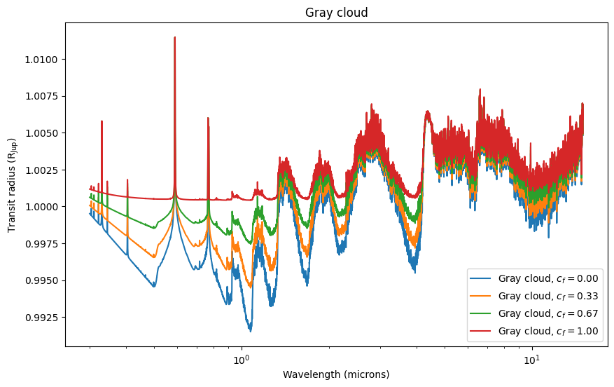
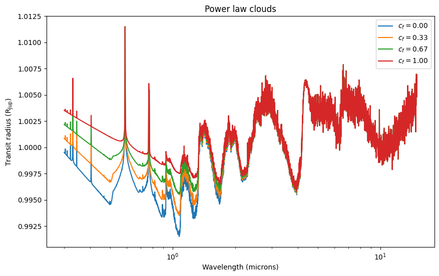
Cloud fraction#

All of the examples above were assuming that the observed section of the planet is fully covered by clouds. While this assumption can be reasonable for some planets (e.g. Venus), clouds can sometimes form patches instead (e.g. Jupiter or the Earth). A way to model this is by using a “cloud fraction” (\(c_f\)) parameter, which combines a clear and a (fully covered) cloudy atmosphere following:

\begin{equation} F = c_f * F_\mathrm{cloudy} + (1 - c_f) * F_\mathrm{clear}. \end{equation}

In petitRADTRANS, the cloud fraction can be set by using the cloud_fraction argument. The following cloud models are affected:

The gray cloud deck.
The power law clouds.
The “physical” clouds.
The arbitrary opacities.

The following opacities or cloud models are not affected by cloud fraction:

The Rayleigh scale factor.
The line opacities.
The CIA opacities.
The non-CIA gas continuum opacities.
The gray opacity (not to be confused with the gray cloud).
The Rayleigh opacities.

Default usage#

Below are examples for each of these cases.

[10]:

cloud_fractions = jnp.linspace(0, 1, 4)

[16]:

# Gray cloud deck
fig, ax = plt.subplots(figsize=(10, 6))

for cloud_fraction in cloud_fractions:
    wavelengths, transit_radii, _ = atmosphere.calculate_transit_radii(
        temperatures=temperatures,
        mass_fractions=mass_fractions,
        mean_molar_masses=mean_molar_masses,
        reference_gravity=reference_gravity,
        planet_radius=planet_radius,
        reference_pressure=reference_pressure,
        opaque_cloud_top_pressure=1e-2,
        cloud_fraction=cloud_fraction,
    )
    ax.plot(wavelengths * 1e4, transit_radii / cst.r_jup_mean, label=rf"Gray cloud, $c_f = {cloud_fraction:.2f}$")

ax.set_xscale("log")
ax.set_xlabel("Wavelength (microns)")
ax.set_ylabel(r"Transit radius ($\rm R_{Jup}$)")
ax.set_title("Gray cloud")
plt.legend()

[16]:

<matplotlib.legend.Legend at 0x31f0cd250>

../../_images/content_notebooks_including_clouds_84_1.png

[6]:

# Power law clouds
fig, ax = plt.subplots(figsize=(10, 6))

for cloud_fraction in cloud_fractions:
    wavelengths, transit_radii, _ = atmosphere.calculate_transit_radii(
        temperatures=temperatures,
        mass_fractions=mass_fractions,
        mean_molar_masses=mean_molar_masses,
        reference_gravity=reference_gravity,
        planet_radius=planet_radius,
        reference_pressure=reference_pressure,
        power_law_opacity_350nm=1e-2,
        power_law_opacity_coefficient=-2,
        cloud_fraction=cloud_fraction,
    )
    ax.plot(wavelengths * 1e4, transit_radii / cst.r_jup_mean, label=rf"$c_f = {cloud_fraction:.2f}$")

ax.set_xscale("log")
ax.set_xlabel("Wavelength (microns)")
ax.set_ylabel(r"Transit radius ($\rm R_{Jup}$)")
ax.set_title("Power law clouds")
plt.legend()

[6]:

<matplotlib.legend.Legend at 0x17fcf7410>

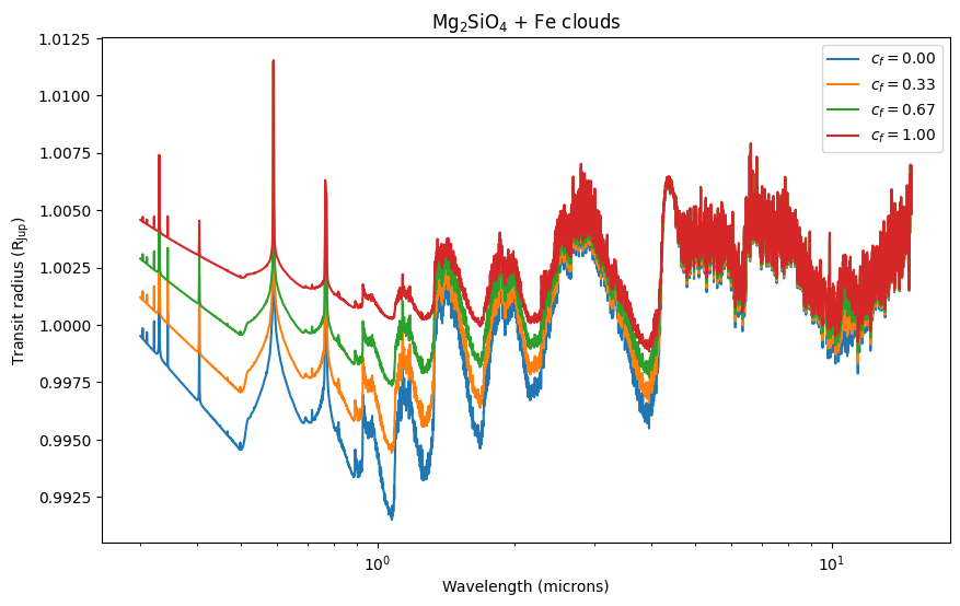
../../_images/content_notebooks_including_clouds_85_1.png

[7]:

# Physical clouds
fig, ax = plt.subplots(figsize=(10, 6))

mass_fractions["Mg2SiO4(s)_crystalline_000__DHS"] = 5e-7 * jnp.ones_like(temperatures)
mass_fractions["Fe(s)_amorphous__Mie"] = 5e-7 * jnp.ones_like(temperatures)

for cloud_fraction in cloud_fractions:
    wavelengths, transit_radii, _ = atmosphere.calculate_transit_radii(
        temperatures=temperatures,
        mass_fractions=mass_fractions,
        mean_molar_masses=mean_molar_masses,
        reference_gravity=reference_gravity,
        planet_radius=planet_radius,
        reference_pressure=reference_pressure,
        eddy_diffusion_coefficients=eddy_diffusion_coefficients,
        cloud_f_sed=cloud_f_sed,
        cloud_particle_radius_distribution_std=cloud_particle_radius_distribution_std,
        cloud_fraction=cloud_fraction,
        patchy_clouds=("Mg2SiO4(s)_crystalline_000__DHS", "Fe(s)_amorphous__Mie")
    )
    ax.plot(wavelengths * 1e4, transit_radii / cst.r_jup_mean, label=rf"$c_f = {cloud_fraction:.2f}$")

ax.set_xscale("log")
ax.set_xlabel("Wavelength (microns)")
ax.set_ylabel(r"Transit radius ($\rm R_{Jup}$)")
ax.set_title(r"Mg$_2$SiO$_4$ + Fe clouds")
plt.legend()

[7]:

<matplotlib.legend.Legend at 0x328fc00e0>

../../_images/content_notebooks_including_clouds_86_1.png

[ ]:

# Arbitrary opacities
fig, ax = plt.subplots(figsize=(10, 6))

mass_fractions["Mg2SiO4(s)_crystalline__DHS"] = 0.0 * jnp.ones_like(temperatures)
mass_fractions["Fe(s)_amorphous__Mie"] = 0.0 * jnp.ones_like(temperatures)

for cloud_fraction in cloud_fractions:
    wavelengths, transit_radii, _ = atmosphere.calculate_transit_radii(
        temperatures=temperatures,
        mass_fractions=mass_fractions,
        mean_molar_masses=mean_molar_masses,
        reference_gravity=reference_gravity,
        planet_radius=planet_radius,
        reference_pressure=reference_pressure,
        additional_absorption_opacities_function=cloud_opas(1e1, 0.5, 4, 0.001, 1),
        cloud_fraction=cloud_fraction,
    )
    ax.plot(wavelengths * 1e4, transit_radii / cst.r_jup_mean, label=rf"$c_f = {cloud_fraction:.2f}$")

ax.set_xscale("log")
ax.set_xlabel("Wavelength (microns)")
ax.set_ylabel(r"Transit radius ($\rm R_{Jup}$)")
ax.set_title(r"Arbitrary opacities")
plt.legend()

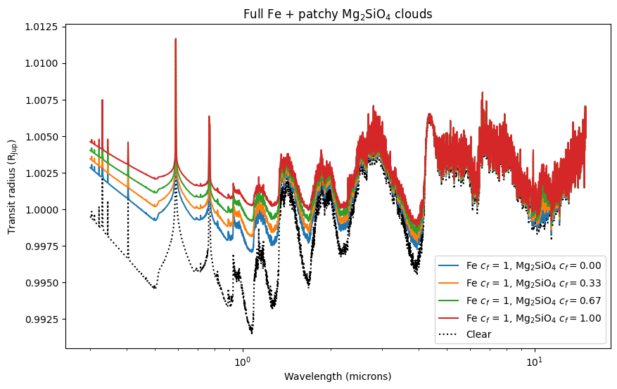
Control which physical clouds are patchy#

It is also possible to control which physical clouds are affected by the cloud fraction. For example, we can imagine a case where a planet is fully covered by deep \(\rm Fe\) clouds, while \(\mathrm{Mg}_2\mathrm{SiO}_4\) clouds form patches in the upper atmosphere. This can be done by using the patchy_clouds argument to list the cloud species that are patchy.

[8]:

# Full Fe + patchy Mg2SiO4
fig, ax = plt.subplots(figsize=(10, 6))

mass_fractions["Mg2SiO4(s)_crystalline__DHS"] = 5e-7 * jnp.ones_like(temperatures)
mass_fractions["Fe(s)_amorphous__Mie"] = 5e-7 * jnp.ones_like(temperatures)

for cloud_fraction in cloud_fractions:
    wavelengths, transit_radii, _ = atmosphere.calculate_transit_radii(
        temperatures=temperatures,
        mass_fractions=mass_fractions,
        mean_molar_masses=mean_molar_masses,
        reference_gravity=reference_gravity,
        planet_radius=planet_radius,
        reference_pressure=reference_pressure,
        eddy_diffusion_coefficients=eddy_diffusion_coefficients,
        cloud_f_sed=cloud_f_sed,
        cloud_particle_radius_distribution_std=cloud_particle_radius_distribution_std,
        cloud_fraction=cloud_fraction,
        patchy_clouds=("Mg2SiO4(s)_crystalline__DHS",),
    )
    ax.plot(
        wavelengths * 1e4,
        transit_radii / cst.r_jup_mean,
        label=rf"Fe $c_f$ = 1, Mg$_2$SiO$_4$ $c_f = {cloud_fraction:.2f}$",
        zorder=3,
    )

ax.plot(wavelengths * 1e4, transit_radii_clear, label=r"Clear", color="K__Allard", ls=":", zorder=2)

ax.set_xscale("log")
ax.set_xlabel("Wavelength (microns)")
ax.set_ylabel(r"Transit radius ($\rm R_{Jup}$)")
ax.set_title(r"Full Fe + patchy Mg$_2$SiO$_4$ clouds")
plt.legend()

/Users/nasedkin/python-packages/petitRADTRANS/petitRADTRANS/radtrans.py:3501: UserWarning: cloud_fraction is less than 1, but there are no patchy clouds. Please add cloud species with partial coverage to 'patchy_clouds'.
  ) = self._init_spectral_function(
/Users/nasedkin/python-packages/petitRADTRANS/petitRADTRANS/radtrans.py:3501: UserWarning: cloud_fraction is less than 1, but there are no patchy clouds. Please add cloud species with partial coverage to 'patchy_clouds'.
  ) = self._init_spectral_function(

---------------------------------------------------------------------------
NameError                                 Traceback (most recent call last)
Cell In[8], line 28
      8     wavelengths, transit_radii, _ = atmosphere.calculate_transit_radii(
      9         temperatures=temperatures,
     10         mass_fractions=mass_fractions,
   (...)
     19         patchy_clouds=("Mg2SiO4(s)_crystalline__DHS",),
     20     )
     21     ax.plot(
     22         wavelengths * 1e4,
     23         transit_radii / cst.r_jup_mean,
     24         label=rf"Fe $c_f$ = 1, Mg$_2$SiO$_4$ $c_f = {cloud_fraction:.2f}$",
     25         zorder=3,
     26     )
---> 28 ax.plot(wavelengths * 1e4, transit_radii_clear, label=r"Clear", color="K__Allard", ls=":", zorder=2)
     30 ax.set_xscale("log")
     31 ax.set_xlabel("Wavelength (microns)")

NameError: name 'transit_radii_clear' is not defined

../../_images/content_notebooks_including_clouds_90_2.png

Emission spectra#

We can use the Radtrans object created above to calculate emission spectra as well. Here we will also generate an instance of pRT with scattering turned on with scattering_in_emission = True, (see “Scattering for Emission Spectra” for an example on how to do this in detail).

[9]:

fig, ax = plt.subplots(figsize=(10, 6))

mass_fractions["Mg2SiO4(s)_crystalline_000__DHS"] = jnp.zeros_like(temperatures)
mass_fractions["Fe(s)_amorphous__Mie"] = jnp.zeros_like(temperatures)

wavelengths, flux, _ = atmosphere.calculate_flux(
    temperatures=temperatures,
    mass_fractions=mass_fractions,
    mean_molar_masses=mean_molar_masses,
    reference_gravity=reference_gravity,
    eddy_diffusion_coefficients=eddy_diffusion_coefficients,
    cloud_f_sed=cloud_f_sed,
    cloud_particle_radius_distribution_std=cloud_particle_radius_distribution_std,
)

ax.plot(wavelengths * 1e4, flux, label="clear, no scattering")

mass_fractions["Mg2SiO4(s)_crystalline_000__DHS"] = 5e-7 * jnp.ones_like(temperatures)
mass_fractions["Fe(s)_amorphous__Mie"] = 5e-7 * jnp.ones_like(temperatures)

wavelengths, flux, _ = atmosphere.calculate_flux(
    temperatures=temperatures,
    mass_fractions=mass_fractions,
    mean_molar_masses=mean_molar_masses,
    reference_gravity=reference_gravity,
    eddy_diffusion_coefficients=eddy_diffusion_coefficients,
    cloud_f_sed=cloud_f_sed,
    cloud_particle_radius_distribution_std=cloud_particle_radius_distribution_std,
)

ax.plot(wavelengths * 1e4, flux, label="cloudy, no scattering")

atmosphere_scat = Radtrans(
    pressures=jnp.logspace(-6, 2, 100),
    line_species=("H2O", "CO-NatAbund", "CH4", "CO2", "Na__NewAllard", "K__Allard"),
    rayleigh_species=("H2", "He"),
    gas_continuum_contributors=("H2--H2", "H2--He"),
    cloud_species=("Mg2SiO4(s)_crystalline_000__DHS", "Fe(s)_amorphous__Mie"),
    wavelength_boundaries=(0.3, 15),
    scattering_in_emission=True,
)

wavelengths, flux, _ = atmosphere_scat.calculate_flux(
    temperatures=temperatures,
    mass_fractions=mass_fractions,
    mean_molar_masses=mean_molar_masses,
    reference_gravity=reference_gravity,
    eddy_diffusion_coefficients=eddy_diffusion_coefficients,
    cloud_f_sed=cloud_f_sed,
    cloud_particle_radius_distribution_std=cloud_particle_radius_distribution_std,
)

ax.plot(wavelengths * 1e4, flux, label="cloudy, scattering")

ax.set_xscale("log")
ax.set_xlabel("Wavelength [microns]")
ax.set_ylabel(r"Planet flux, $F_{\lambda}$ [erg cm$^{-2}$ s$^{-1}$ cm$^{-1}$]")

ax.legend()

plt.show()

../../_images/content_notebooks_including_clouds_93_1.png

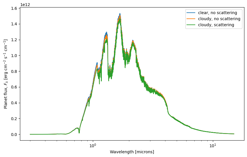
Here we plotted the clear spectrum, neglecting the cloud opacity, the cloudy spectrum only considering the absorption of the cloud particles, and the cloudy spectrum with scattering, using the scattering version of pRT.

Scattering and petitRADTRANS: remember that scattering is included for emission spectra in petitRADTRANS only if requested specifically when generating the Radtrans object, as it increases the runtime (see “Scattering for Emission Spectra” for an example how to do this).

Standard flux units: before pRT3 flux was accessed as atmosphere.flux after running atmosphere.calc_flux(), which contained flux as \(F_\nu\), so in units of erg cm\(^{-2}\) s\(^{-1}\) Hz\(^{-1}\). pRT’s calculate_flux() method now returns wavelength and flux as \(F_\lambda\) in its standard setting, so flux in erg cm\(^{-2}\) s\(^{-1}\) cm\(^{-1}\). To return frequencies and \(F_\nu\), instead of wavelengths and \(F_\lambda\), please set the keyword frequencies_to_wavelengths=False when calling calculate_flux().

`SpectralModel`#

To include cloud models in a SpectralModel object, simply replace the cloud models arguments that you would use with Radtrans with model parameters. Below is an example with physical clouds. The other ways to add cloud models are commented.

[23]:

spectral_model = SpectralModel(
    # Cloud parameters
    eddy_diffusion_coefficients=eddy_diffusion_coefficients,
    cloud_f_sed=cloud_f_sed,
    cloud_particle_radius_distribution_std=cloud_particle_radius_distribution_std,
    cloud_fraction=1.0,
    # Other cloud parameters
    # opaque_cloud_top_pressure=1e-2,
    # haze_factor=10,
    # power_law_opacity_350nm=power_law_opacity_350nm,
    # power_law_opacity_coefficient=power_law_opacity_coefficient,
    # additional_absorption_opacities_function=cloud_opas,
    # Radtrans parameters
    pressures=jnp.logspace(-6, 2, 100),
    line_species=("H2O", "CO-NatAbund", "CH4", "CO2", "Na__NewAllard", "K__Allard"),
    rayleigh_species=["H2", "He"],
    gas_continuum_contributors=["H2--H2", "H2--He"],
    cloud_species=["Mg2SiO4(s)_crystalline_000__DHS", "Fe(s)_amorphous__Mie"],
    patchy_clouds=("Mg2SiO4(s)_crystalline_000__DHS",),
    wavelength_boundaries=(0.3, 15),
    # Model parameters
    # Planet parameters
    planet_radius=planet_radius,
    reference_gravity=reference_gravity,
    reference_pressure=reference_pressure,
    # Temperature profile parameters
    temperature_profile_mode="guillot",
    temperature=equilibrium_temperature,
    intrinsic_temperature=intrinsic_temperature,
    guillot_temperature_profile_infrared_mean_opacity_solar_metallicity=infrared_mean_opacity,
    guillot_temperature_profile_gamma=gamma,
    # Mass fractions
    imposed_mass_fractions={
        "H2O": 1e-3,
        "CO-NatAbund": 1e-2,
        "CH4": 1e-6,
        "CO2": 1e-5,
        "Na__NewAllard": 1e-5,
        "K__Allard": 1e-6,
        "Mg2SiO4(s)_crystalline_000__DHS": 5e-7,
        "Fe(s)_amorphous__Mie": 5e-7,
    },
    filling_species={"H2": 37, "He": 12},
)

[24]:

# Full Fe + patchy Mg2SiO4
fig, ax = plt.subplots(figsize=(10, 6))

for cloud_fraction in cloud_fractions:
    spectral_model.model_parameters["cloud_fraction"] = cloud_fraction
    wavelengths, transit_radii = spectral_model.calculate_spectrum(mode="transmission")
    ax.plot(
        wavelengths[0] * 1e4,
        transit_radii[0] / cst.r_jup_mean,
        label=rf"Fe $c_f$ = 1, Mg$_2$SiO$_4$ $c_f = {cloud_fraction:.2f}$",
        zorder=3,
    )

ax.plot(wavelengths[0] * 1e4, transit_radii_clear, label=r"Clear", color="k", ls=":", zorder=2)

ax.set_xscale("log")
ax.set_xlabel("Wavelength (microns)")
ax.set_ylabel(r"Transit radius ($\rm R_{Jup}$)")
ax.set_title(r"Full Fe + patchy Mg$_2$SiO$_4$ clouds")
plt.legend()

[24]:

<matplotlib.legend.Legend at 0x3d076c080>

../../_images/content_notebooks_including_clouds_100_1.png

[ ]:

Including clouds

Contents

Including clouds#

Gray cloud deck#

Scaled Rayleigh scattering#

Powerlaw cloud models#

Condensate clouds from real optical constants#

Setting the cloud particles size#

Calculating the cloud particles size#

Fixed settling parameter#

Vertically variable settling parameter#

Hansen Distribution Clouds#

Defining arbitrary opacity functions (can be used to parameterize clouds)#

Cloud fraction#

Default usage#

Control which physical clouds are patchy#

Emission spectra#

SpectralModel#

`SpectralModel`#