Chemistry in petitRADTRANS

from jax import config
config.update("jax_enable_x64", True)

import jax.numpy as jnp
import numpy as np
import matplotlib.pyplot as plt

from petitRADTRANS.temperature_profiles import guillot_global_temperature_profile
from petitRADTRANS.chemistry.pre_calculated_chemistry import PreCalculatedEquilibriumChemistryTable

Interpolated chemical equilibrium

To set the abundance of atmospheric absorbers we need to make assumptions on the atmospheric composition. When fitting exoplanet spectra, one option is to let the composition float freely, and tune it to values that best fit the data. Alternatively, one can turn to chemical models that calculate atmospheric abundances from the atmospheric elemental composition and the chemical reactions that link these elements and chemical reactant species. In the atmosphere of an exoplanet, which is inherently three-dimensional and dynamic, mixing and advection processes complicate this picture, because the chemical abundances inferred from spectra are not necessarily representative of the pressures and temperatures probed locally by the observation. In addition, the radiation field of the host star may influence the abundance and therefore opacity structure of the atmosphere, by dissociating or ionizing chemical species, which can then give rise to photochemically produced chemical species, or form photochemical hazes. In this picture, using chemical equilibrium abundances, which means the steady state chemical composition of the atmosphere when treating its layers as isolated and independent (no advection/mixing/photochemistry), appears unwise.

Yet, calculating chemical equilibrium abundances may still serve as a useful starting point for initializing abundances in planetary atmospheres. In certain conditions, for example for planets hot enough such that mixing is negligible, chemical equilibrium abundances can even be sufficient to accurately describe the abundances in the atmospheric region probed by observations.

Here we show how to use our chemistry.pre_calculated_chemistry subpackage. This package interpolates the abundances of the most important (i.e., spectrally active and abundant) species from a large chemical equilibrium table as a function of pressure, temperature, metallicity [Fe/H] (where [Fe/H]=0 is solar) and cabon-to-oxygen number ratio (C/O). A C/O \(\sim 0.55\) is the solar value, see, for example, Asplund et al. (2009).

chemistry.pre_calculated_chemistry also contains a simple quenching implementation. This means that a quench pressure can be specified below which (so for higher atmospheric altitudes) the abundances of H\(_2\)O, CH\(_4\) and CO are taken to be constant, following the reasoning in, for example, Zahnle & Marley (2014). In principle, you can quench even more species by manually setting their abundances constant above a given altitude, once you have the abundance dictionary returned by chemistry.pre_calculated_chemistry.

The abundance table in chemistry.pre_calculated_chemistry has been calculated with easyCHEM, which is our open-source Python package for calculating chemical equilibrium abundances. easyCHEM has been first described in Mollière et al. (2017), and it implements the methods described for NASA’s CEA code, see Gordon & McBride (1994). easyCHEM has been benchmarked as the chemical equilibrium tool of petitCODE in Baudino et al. (2017).

The grid dimensions of the chemistry.pre_calculated_chemistry abundance table are \(T \in [60, 4000]~{\rm K}\), with 100 equidistant temperature points, \(P \in [10^{-8}, 1000]~{\rm bar}\), with 100 pressure points spaced equidistantly in log space, \({\rm C/O} \in [0.1, 1.6]\), with 20 equidistant points, and \({\rm [Fe/H]} \in [-1,3]\), with 40 equidistant points. In chemistry.pre_calculated_chemistry the C/O is changed by varying the oxygen content after all metal species (so all elements except for H and He) have been scaled by \(10^{\rm [Fe/H]}\). The total list of reactant species included was H, H\(_2\), He, O, C, N, Mg, Si, Fe, S, Al, Ca, Na, Ni, P, K, Ti, CO, OH, SH, N\(_2\), O\(_2\), SiO, TiO, SiS, H\(_2\)O, C\(_2\), CH, CN, CS, SiC, NH, SiH, NO, SN, SiN, SO, S\(_2\), C\(_2\)H, HCN, C\(_2\)H\(_2\) (acetylene), CH\(_4\), AlH, AlOH, Al\(_2\)O, CaOH, MgH, Mg, OH, PH\(_3\), CO\(_2\), TiO\(_2\), Si\(_2\)C, SiO\(_2\), FeO, NH\(_2\), NH\(_3\), CH\(_2\), CH\(_3\), H\(_2\)S, VO, VO\(_2\), NaCl, KCl, e-, H+, H-, Na+, K+, PH\(_2\), P\(_2\), PS, PO, P\(_4\)O\(_6\), PH, V, FeH, VO(c), VO(L), MgSiO\(_3\)(c), SiC(c), Fe(c), Na\(_2\)S(c), KCL(c), Fe(L), SiC(L), MgSiO\(_3\)(L), H\(_2\)O(L), H\(_2\)O(c), TiO(c), TiO(L), TiO\(_2\)(c), TiO\(_2\)(L), H\(_3\)PO\(_4\)(c), H\(_3\)PO\(_4\)(L), where (c) stands for solid and (L) for liquid species. To conserve space only the mass fractions of the following species are tabulated for use in chemistry.pre_calculated_chemistry: H\(_2\), He, CO, H\(_2\)O, HCN, C\(_2\)H\(_2\) (acetylene), CH\(_4\), PH\(_3\), CO\(_2\), NH\(_3\), H\(_2\)S, VO, TiO, Na, K, SiO, e-, H-, H, FeH, MMW, nabla_ad. MMW denotes the mean molar mass in the atmosphere. nabla_ad is the moist adiabatic lapse rate \(\nabla_{\rm ad} = (\partial {\rm ln}T/\partial {\rm ln}P)_{\rm ad}\), determined as described in Mollière et al. (2020).

Abundances in chemistry.pre_calculated_chemistry are in units of mass fractions, not number fractions (aka volume mixing ratios, VMRs). You can convert between mass fractions and VMRs by using \begin{equation} X_i = \frac{\mu_i}{\mu}n_i, \end{equation} where \(X_i\) is the mass fraction of species \(i\), \(\mu_i\) the molar mass of a molecule/atom/ion/… of species \(i\), \(\mu\) is the atmospheric mean molar mass, and \(n_i\) is the VMR of species \(i\). This is implemented in petitRADTRANS.chemistry.utils.mass_fractions2volume_mixing_ratios() and petitRADTRANS.chemistry.utils.volume_mixing_ratios2mass_fractions().

Here we will give some examples for how to interpolate chemical abundances using chemistry.pre_calculated_chemistry.

plt.rcParams["figure.figsize"] = (10, 6)

chem = PreCalculatedEquilibriumChemistryTable()

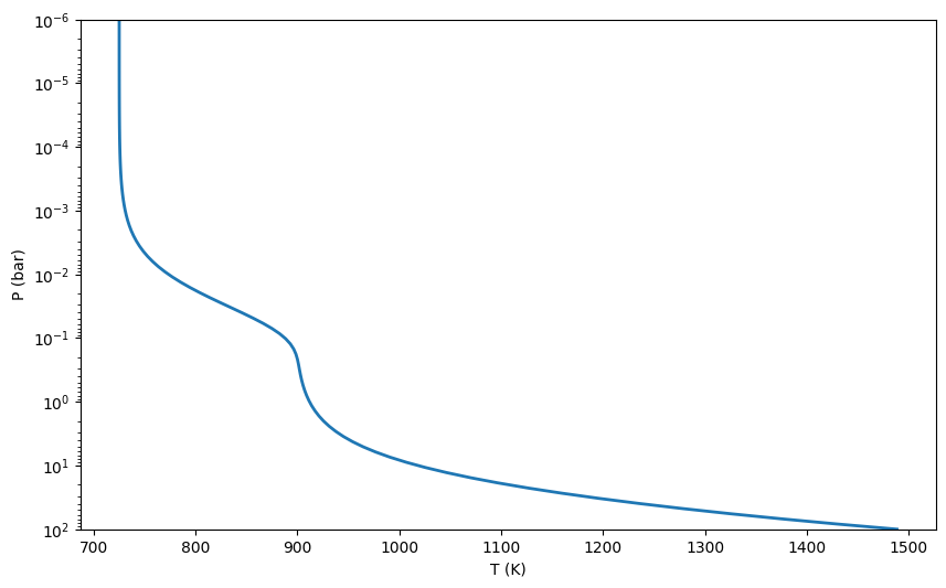
Next, we define an atmospheric temperature and abundance structure, following an example similar to what is shown in “Getting Started”.

pressures = jnp.logspace(-6, 2, 100)

reference_gravity = 10**2.45
infrared_mean_opacity = 0.01
gamma = 0.4
intrinsic_temperature = 200
equilibrium_temperature = 800

temperatures = guillot_global_temperature_profile(
    pressures=pressures,
    infrared_mean_opacity=infrared_mean_opacity,
    gamma=gamma,
    gravities=reference_gravity,
    intrinsic_temperature=intrinsic_temperature,
    equilibrium_temperature=equilibrium_temperature,
)

plt.plot(temperatures, pressures, linewidth = 2)
plt.yscale("log")
plt.ylim([1e2, 1e-6])
plt.xlabel("T (K)")
plt.ylabel("P (bar)")

Text(0, 0.5, 'P (bar)')

Now we calculate the abundances. Note that the input parameters temperature, pressure, [Fe/H] and C/O are all arrays, and must be defined at every layer, but usually C/O and [Fe/H] are not vertically varying in the atmosphere. Here we chose a solar metallicity and C/O.

co_ratios = 0.55 * np.ones_like(pressures)
log10_metallicities = 0.0 * np.ones_like(pressures)

mass_fractions, mean_molar_mass, nabla_ad = chem.interpolate_mass_fractions(
    co_ratios=co_ratios,
    log10_metallicities=log10_metallicities,
    temperatures=temperatures,
    pressures=pressures,
    full=True,
)

Loading chemical equilibrium chemistry table from file '/Users/nasedkin/python-packages/petitRADTRANS/input_data/pre_calculated_chemistry/equilibrium_chemistry/equilibrium_chemistry.chemtable.petitRADTRANS.h5'... Done.

This is what the full boolean flag stands for (nominal value is False):

full:
    if True, return the pre-calculated mean molar mass and logarithmic derivative of temperature with
    respect to pressure in the adiabatic case (nabla_ad) in addition to the pre-calculated mass fractions

Quenching is turned on by using the optional carbon_quench_pressure keyword argument (nominal value is None):

carbon_quench_pressure:
    (bar) pressure at which to put a simplistic carbon-bearing species quenching

for pressures_bar < carbon_quench_pressure the abundances of H\(_2\)O, CH\(_4\) and CO are then taken to be constant.

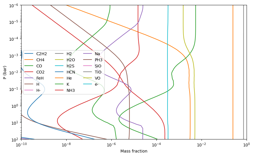
Lets plot the abundances:

plt.yscale("log")
plt.xscale("log")
plt.ylim([100, 1e-6])
plt.xlim([1e-10, 1])

for species in mass_fractions.keys():
    plt.plot(mass_fractions[species], pressures, label=species)

plt.legend(loc="best", ncol=3)
plt.xlabel("Mass fraction")
plt.ylabel("P (bar)")

Text(0, 0.5, 'P (bar)')

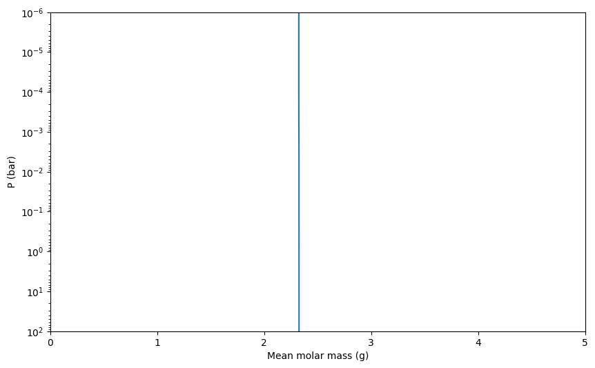
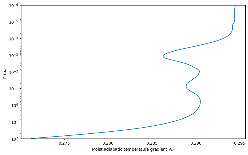
Also the MMW and adiabatic temperature gradient are accessible, where the former turns out to be vertically constant for this atmosphere:

plt.yscale("log")
plt.ylim([100, 1e-6])
plt.xlim([0, 5])

plt.plot(mean_molar_mass, pressures, label=species)

plt.xlabel("Mean molar mass (g)")
plt.ylabel("P (bar)")

Text(0, 0.5, 'P (bar)')

plt.yscale("log")
plt.ylim([100, 1e-6])

plt.plot(nabla_ad, pressures, label=species)

plt.xlabel(r"Moist adiabatic temperature gradient $\nabla_{\rm ad}$")
plt.ylabel("P (bar)")

Text(0, 0.5, 'P (bar)')

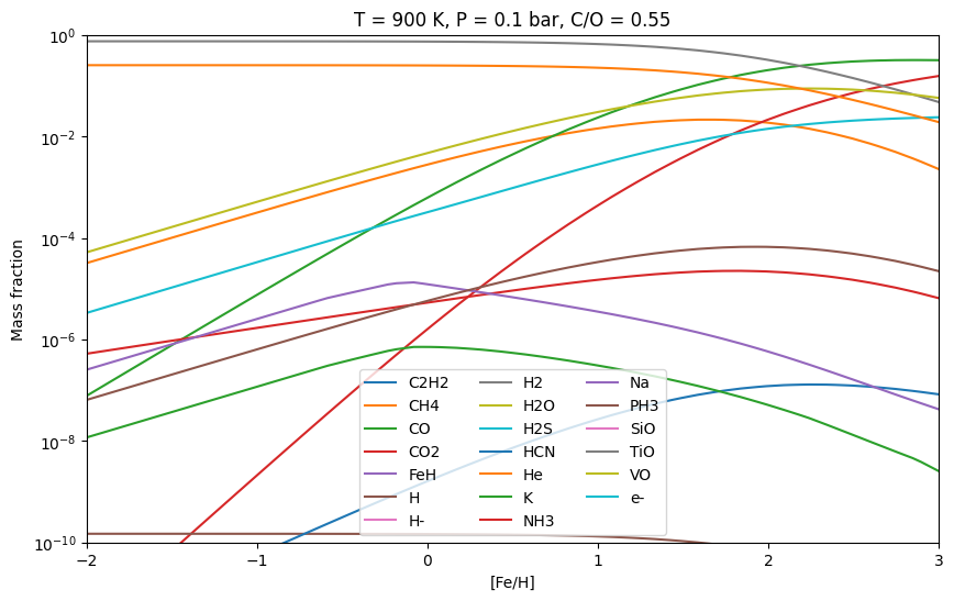
As a test, we can also plot abundances at a given pressure, temperature, C/O, as a function of metallicity:

log10_metallicities = np.linspace(-2, 3, 100)
pressures_constant = np.ones_like(log10_metallicities) * 1e-1
temperatures_constant = np.ones_like(log10_metallicities) * 900
co_ratios = 0.55 * np.ones_like(log10_metallicities)

mass_fractions, mean_molar_mass, nabla_ad = chem.interpolate_mass_fractions(
    co_ratios=co_ratios,
    log10_metallicities=log10_metallicities,
    temperatures=temperatures_constant,
    pressures=pressures_constant,
    full=True,
)

plt.yscale("log")
plt.ylim([1e-10, 1])
plt.xlim([-2, 3])

for species in mass_fractions.keys():
    plt.plot(log10_metallicities, mass_fractions[species], label=species)

plt.legend(loc="best", ncol=3)
plt.ylabel("Mass fraction")
plt.xlabel("[Fe/H]")
plt.title("T = 900 K, P = 0.1 bar, C/O = 0.55")

Text(0.5, 1.0, 'T = 900 K, P = 0.1 bar, C/O = 0.55')

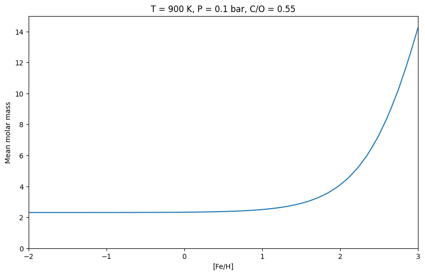
This is the mean molar mass as a function of metallicity:

plt.xlim([-2, 3])
plt.ylim([0, 15])

plt.plot(log10_metallicities, mean_molar_mass)

plt.ylabel("Mean molar mass")
plt.xlabel("[Fe/H]")
plt.title("T = 900 K, P = 0.1 bar, C/O = 0.55")

Text(0.5, 1.0, 'T = 900 K, P = 0.1 bar, C/O = 0.55')

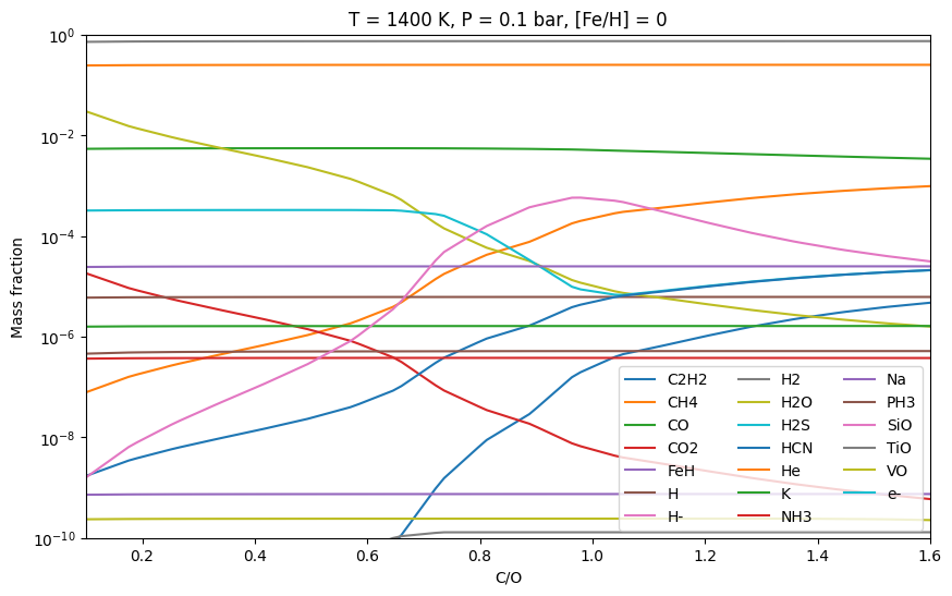
Next we plot the mass fractions as a function of the C/O ratio, at solar metallicity:

co_ratios = np.linspace(0.1, 1.6, 100)
log10_metallicities = 0.0 * np.ones_like(co_ratios)
pressures_constant = np.ones_like(co_ratios) * 1e-1
temperatures_constant = np.ones_like(co_ratios) * 1400

mass_fractions, mean_molar_mass, nabla_ad = chem.interpolate_mass_fractions(
    co_ratios=co_ratios,
    log10_metallicities=log10_metallicities,
    temperatures=temperatures_constant,
    pressures=pressures_constant,
    full=True,
)

plt.yscale("log")
plt.ylim([1e-10, 1])
plt.xlim([0.1, 1.6])

for species in mass_fractions.keys():
    plt.plot(co_ratios, mass_fractions[species], label=species)

plt.legend(loc="lower right", ncol=3)
plt.ylabel("Mass fraction")
plt.xlabel("C/O")
plt.title("T = 1400 K, P = 0.1 bar, [Fe/H] = 0")

Text(0.5, 1.0, 'T = 1400 K, P = 0.1 bar, [Fe/H] = 0')

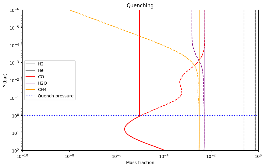
Finally, we show an example with quenching here, assuming that the CH\(_4\), H\(_2\)O and CO abundances are constant in for pressures below 1 bar. We will use the temperature structure from above again.

# Nominal case:
co_ratios = 0.55 * np.ones_like(pressures)
log10_metallicities = 0.0 * np.ones_like(pressures)

mass_fractions = chem.interpolate_mass_fractions(
    co_ratios=co_ratios, log10_metallicities=log10_metallicities, temperatures=temperatures, pressures=pressures
)

# Quenching case:
mass_fractions_quench = chem.interpolate_mass_fractions(
    co_ratios=co_ratios,
    log10_metallicities=log10_metallicities,
    temperatures=temperatures,
    pressures=pressures,
    carbon_quench_pressure=1.0,
)

plt.yscale("log")
plt.xscale("log")
plt.ylim([100, 1e-6])
plt.xlim([1e-10, 1])

plt.plot(mass_fractions["H2"], pressures, linestyle="--", color="black")
plt.plot(mass_fractions_quench["H2"], pressures, label="H2", linestyle="-", color="black")
plt.plot(mass_fractions["He"], pressures, linestyle="--", color="gray")
plt.plot(mass_fractions_quench["He"], pressures, label="He", linestyle="-", color="gray")
plt.plot(mass_fractions["CO"], pressures, linestyle="--", color="red")
plt.plot(mass_fractions_quench["CO"], pressures, label="CO", linestyle="-", color="red")
plt.plot(mass_fractions["H2O"], pressures, linestyle="--", color="purple")
plt.plot(mass_fractions_quench["H2O"], pressures, label="H2O", linestyle="-", color="purple")
plt.plot(mass_fractions["CH4"], pressures, linestyle="--", color="orange")
plt.plot(mass_fractions_quench["CH4"], pressures, label="CH4", linestyle="-", color="orange")

plt.axhline(1.0, color="blue", linestyle=":", label="Quench pressure")

plt.legend(loc="best", ncol=1)
plt.xlabel("Mass fraction")
plt.ylabel("P (bar)")
plt.title("Quenching")

Text(0.5, 1.0, 'Quenching')

The get_abundances function

petitRADTRANS.chemistry.core.get_abundances is the high-level helper that assembles the gas and cloud composition for a pressure-temperature profile. This is the standard method for calculating the chemistry in the retrieval module. It returns exactly the objects that the radiative-transfer path needs:

mass_fractions, mean_molar_mass, pressure_indices, p_bases = get_abundances(
    pressures=pressures,
    temperatures=temperatures,
    parameters=parameters,
    line_species=("H2O", "CO", "CH4", "CO2"),
    cloud_species=(),
)

The most important inputs are:

• pressures and temperatures: arrays on the same vertical grid.

• parameters: the chemistry controls. If it only contains explicit species abundances such as "H2O": -3.5, the function runs in free-chemistry mode. If it contains metallicity and carbon-to-oxygen controls such as "Fe/H" and "C/O", or use_equilibrium_chemistry=True, it uses the built-in equilibrium table.

• line_species: the gas species whose abundances should be prepared for the model.

• cloud_species: optional condensates. If this is empty, p_bases is also empty.

• filling_species is optional. If omitted, the remaining atmospheric mass is filled with an H2/He background.

A useful feature is that equilibrium and free chemistry can be combined: if equilibrium chemistry is enabled and you also pass explicit species abundances, the explicit species override the equilibrium table while the remaining species still come from equilibrium. Negative abundance inputs are interpreted as log10 mass fractions, so "H2O": -3.5 means an H2O mass fraction of 10**-3.5.

from petitRADTRANS.chemistry.core import get_abundances

example_line_species = ("H2O", "CO", "CH4", "CO2")
example_cloud_species = ()

free_parameters = {
    "H2O": -3.5,
    "CO": -4.5,
    "CH4": -6.0,
}

equilibrium_parameters = {
    "Fe/H": 0.0,
    "C/O": 0.55,
    "use_equilibrium_chemistry": True,
}

mixed_parameters = {
    "Fe/H": 0.0,
    "C/O": 0.55,
    "use_equilibrium_chemistry": True,
    "H2O": -3.5,
    "CO": -4.5,
}

free_abundances, free_mean_molar_mass, free_pressure_indices, free_p_bases = get_abundances(
    pressures=pressures,
    temperatures=temperatures,
    parameters=free_parameters,
    line_species=example_line_species,
    cloud_species=example_cloud_species,
)

equilibrium_abundances, equilibrium_mean_molar_mass, equilibrium_pressure_indices, equilibrium_p_bases = get_abundances(
    pressures=pressures,
    temperatures=temperatures,
    parameters=equilibrium_parameters,
    line_species=example_line_species,
    cloud_species=example_cloud_species,
)

mixed_abundances, mixed_mean_molar_mass, mixed_pressure_indices, mixed_p_bases = get_abundances(
    pressures=pressures,
    temperatures=temperatures,
    parameters=mixed_parameters,
    line_species=example_line_species,
    cloud_species=example_cloud_species,
)

print("Returned objects from get_abundances:")
print("  available species in mass_fractions:", sorted(mixed_abundances.keys()))
print("  mean_molar_mass shape:", mixed_mean_molar_mass.shape)
print("  pressure_indices unchanged:", np.array_equal(np.asarray(mixed_pressure_indices), np.arange(pressures.size)))
print("  cloud bases:", mixed_p_bases)

Loading chemical equilibrium chemistry table from file '/Users/nasedkin/python-packages/petitRADTRANS/input_data/pre_calculated_chemistry/equilibrium_chemistry/equilibrium_chemistry.chemtable.petitRADTRANS.h5'... Done.
Returned objects from get_abundances:
  available species in mass_fractions: ['C2H2', 'CH4', 'CO', 'CO2', 'FeH', 'H', 'H-', 'H2', 'H2O', 'H2S', 'HCN', 'He', 'K', 'NH3', 'Na', 'PH3', 'SiO', 'TiO', 'VO', 'e-']
  mean_molar_mass shape: (100,)
  pressure_indices unchanged: True
  cloud bases: {}

The three calls above use the same pressure-temperature profile but different chemistry controls:

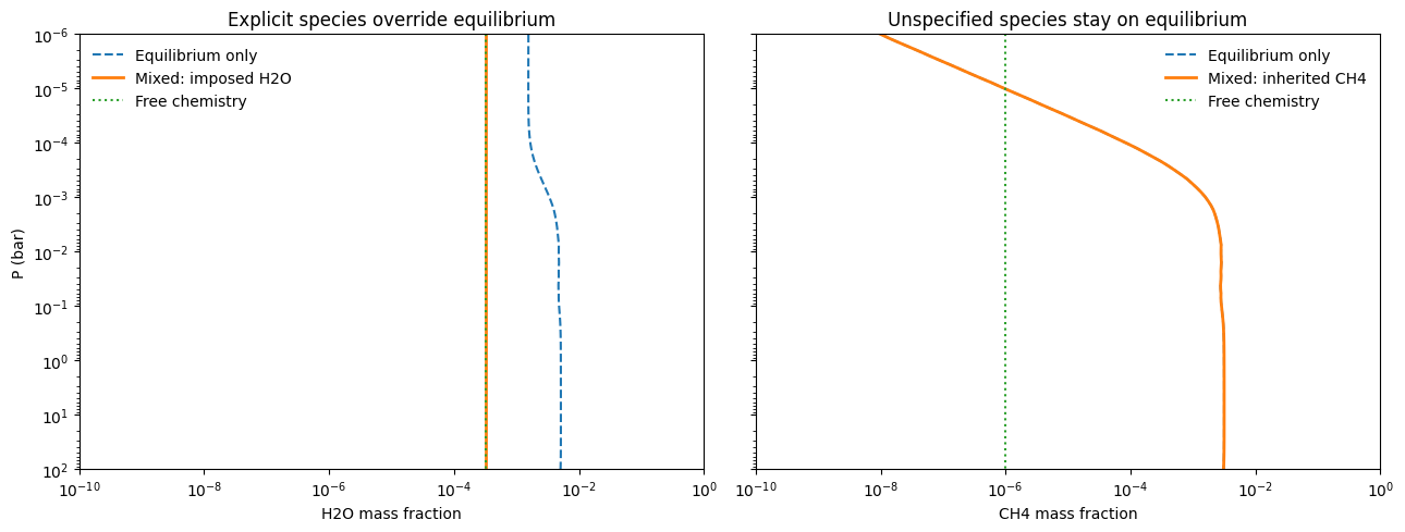
• free_parameters only sets explicit species abundances, so every listed absorber is treated as free chemistry.

• equilibrium_parameters uses the pre-calculated equilibrium table for all requested species.

• mixed_parameters combines both approaches: H2O and CO are imposed explicitly, while CH4, CO2, H2, and He are still taken from the equilibrium solution and the default atmospheric filling.

In the next plot, the H2O profile changes because it is overridden explicitly in the mixed case, while CH4 stays on top of the equilibrium solution because we did not override it.

fig, axes = plt.subplots(1, 2, figsize=(13, 5), sharey=True)

axes[0].plot(np.asarray(equilibrium_abundances["H2O"]), np.asarray(pressures), linestyle="--", label="Equilibrium only")
axes[0].plot(np.asarray(mixed_abundances["H2O"]), np.asarray(pressures), linewidth=2, label="Mixed: imposed H2O")
axes[0].plot(np.asarray(free_abundances["H2O"]), np.asarray(pressures), linestyle=":", label="Free chemistry")
axes[0].set_xscale("log")
axes[0].set_yscale("log")
axes[0].set_ylim([100, 1e-6])
axes[0].set_xlim([1e-10, 1])
axes[0].set_xlabel("H2O mass fraction")
axes[0].set_ylabel("P (bar)")
axes[0].set_title("Explicit species override equilibrium")
axes[0].legend(frameon=False)

axes[1].plot(np.asarray(equilibrium_abundances["CH4"]), np.asarray(pressures), linestyle="--", label="Equilibrium only")
axes[1].plot(np.asarray(mixed_abundances["CH4"]), np.asarray(pressures), linewidth=2, label="Mixed: inherited CH4")
axes[1].plot(np.asarray(free_abundances["CH4"]), np.asarray(pressures), linestyle=":", label="Free chemistry")
axes[1].set_xscale("log")
axes[1].set_yscale("log")
axes[1].set_ylim([100, 1e-6])
axes[1].set_xlim([1e-10, 1])
axes[1].set_xlabel("CH4 mass fraction")
axes[1].set_title("Unspecified species stay on equilibrium")
axes[1].legend(frameon=False)

fig.tight_layout()