Analysis tools#

Before we start, we create an atmospheric setup case based on the “Getting Started” example:

First setting up a Radtrans object:

[1]:

import matplotlib.pyplot as plt
import numpy as np

from petitRADTRANS import physical_constants as cst
from petitRADTRANS.radtrans import Radtrans

atmosphere = Radtrans(
    pressures=np.logspace(-6, 3, 100),
    line_species=[
        'H2O',
        'CO-NatAbund',
        'CH4',
        'CO2',
        'Na__Burrows',
        'K__Burrows'
    ],
    rayleigh_species=['H2', 'He'],
    gas_continuum_contributors=['H2-H2', 'H2-He'],
    wavelength_boundaries=[0.3, 15]
)

Loading Radtrans opacities...
Loading line opacities of species 'H2O' from file '/home/dblain/petitRADTRANS/input_data/opacities/lines/correlated_k/H2O/1H2-16O/1H2-16O__HITEMP.R1000_0.1-250mu.ktable.petitRADTRANS.h5'... Done.
Loading line opacities of species 'CO-NatAbund' from file '/home/dblain/petitRADTRANS/input_data/opacities/lines/correlated_k/CO/C-O-NatAbund/C-O-NatAbund__HITEMP.R1000_0.1-250mu.ktable.petitRADTRANS.h5'... Done.
Loading line opacities of species 'CH4' from file '/home/dblain/petitRADTRANS/input_data/opacities/lines/correlated_k/CH4/12C-1H4/12C-1H4__YT34to10.R1000_0.3-50mu.ktable.petitRADTRANS.h5'... Done.
Loading line opacities of species 'CO2' from file '/home/dblain/petitRADTRANS/input_data/opacities/lines/correlated_k/CO2/12C-16O2/12C-16O2__UCL-4000.R1000_0.3-50mu.ktable.petitRADTRANS.h5'... Done.
Loading line opacities of species 'Na__Burrows' from file '/home/dblain/petitRADTRANS/input_data/opacities/lines/correlated_k/Na/23Na/23Na__Burrows.R1000_0.1-250mu.ktable.petitRADTRANS.h5'... Done.
Loading line opacities of species 'K__Burrows' from file '/home/dblain/petitRADTRANS/input_data/opacities/lines/correlated_k/K/39K/39K__Burrows.R1000_0.1-250mu.ktable.petitRADTRANS.h5'... Done.
Successfully loaded all line opacities
Loading CIA opacities for H2-H2 from file '/home/dblain/petitRADTRANS/input_data/opacities/continuum/collision_induced_absorptions/H2--H2/H2--H2-NatAbund/H2--H2-NatAbund__BoRi.R831_0.6-250mu.ciatable.petitRADTRANS.h5'... Done.
Loading CIA opacities for H2-He from file '/home/dblain/petitRADTRANS/input_data/opacities/continuum/collision_induced_absorptions/H2--He/H2--He-NatAbund/H2--He-NatAbund__BoRi.DeltaWavenumber2_0.5-500mu.ciatable.petitRADTRANS.h5'... Done.
Successfully loaded all CIA opacities
Successfully loaded all opacities

Units in petitRADTRANS: all units inside petitRADTRANS are in cgs. However, when interfacing with the code, you are expected to provide pressures in bars (more intuitive). Pressures will be converted to cgs units within the code.

And the atmospheric parameters:

[2]:

from petitRADTRANS.physics import temperature_profile_function_guillot_global

planet_radius = 1 * cst.r_jup_mean
reference_gravity = 10 ** 3.5
reference_pressure = 0.01

pressures = atmosphere.pressures * 1e-6 # cgs to bar
infrared_mean_opacity = 0.01
gamma = 0.4
intrinsic_temperature = 200
equilibrium_temperature = 1500

temperatures = temperature_profile_function_guillot_global(
    pressures=pressures,
    infrared_mean_opacity=infrared_mean_opacity,
    gamma=gamma,
    gravities=reference_gravity,
    intrinsic_temperature=intrinsic_temperature,
    equilibrium_temperature=equilibrium_temperature
)

mass_fractions = {
    'H2': 0.74 * np.ones(temperatures.size),
    'He': 0.24 * np.ones(temperatures.size),
    'H2O': 1e-3 * np.ones(temperatures.size),
    'CO-NatAbund': 1e-2 * np.ones(temperatures.size),
    'CO2': 1e-4 * np.ones(temperatures.size),
    'CH4': 1e-5 * np.ones(temperatures.size),
    'Na__Burrows': 1e-4 * np.ones(temperatures.size),
    'K__Burrows': 1e-6 * np.ones(temperatures.size)
}

#  2.33 is a typical value for H2-He dominated atmospheres
mean_molar_masses = 2.33 * np.ones_like(temperatures)

Abundances in petitRADTRANS: abundances in pRT are in units of mass fractions, not number fractions (aka volume mixing ratio, VMR). One can convert between mass fractions and VMRs by using \begin{equation} X_i = \frac{\mu_i}{\mu}n_i, \end{equation} where \(X_i\) is the mass fraction of species \(i\), \(\mu_i\) the molar mass of a molecule/atom/ion/… of species \(i\), \(\mu\) is the atmospheric mean molar mass, and \(n_i\) is the VMR of species \(i\). This is implemented in petitRADTRANS.chemistry.utils.mass_fractions2volume_mixing_ratios() and petitRADTRANS.chemistry.utils.volume_mixing_ratios2mass_fractions().

Transmission contribution functions#

We calculate the transmission spectrum in the usual way, this time setting the return_contribution = True keyword argument, however. This will additionally measure the contribution of the different layers, by calculating as many transmission spectra as there are layers, iteratively turning off the opacity in one layer only. The difference to the nominal transmission spectrum then measures the influence of the respective layers. Note that calculating the contribution function will increase the computation time considerably. The formal definition of the contribution function is (Mollière et al. 2019):

\begin{equation} C_{\rm tr}^{i} = \frac{R_{\rm nom}^2-R^2(\kappa_i=0)}{\sum_{j=1}^{N_{\rm L}}\left[R_{\rm nom}^2-R^2(\kappa_j=0)\right]}, \end{equation}

where \(R_{\rm nom}\) is the nominal transmission radius of the planet and \(R(\kappa_i=0)\) is the transmission radius obtained from setting the opacity in the \(i\)th layer to zero. \(N_{\rm L}\) is the number of atmospheric layers.

Now, to the contribution function calculation (this can take a couple of minutes):

[3]:

%%time
wavelengths, transit_radii, additional_outputs = atmosphere.calculate_transit_radii(
    temperatures=temperatures,
    mass_fractions=mass_fractions,
    mean_molar_masses=mean_molar_masses,
    reference_gravity=reference_gravity,
    planet_radius=planet_radius,
    reference_pressure=reference_pressure,
    return_contribution=True
)

CPU times: user 2min 15s, sys: 4.87 s, total: 2min 20s
Wall time: 2min 13s

Transmission contribution functions can also be obtained with a SpectralModel object, using e.g.:

spectral_model = SpectralModel(...)
spectral_model.model_parameters['return_contribution'] = True  # can also be set during the instantiation
wavelengths, transit_radii, additional_outputs = spectral_model.calculate_spectrum(
    mode='transmission',
    return_additional_outputs=True
)

The transmission contribution function is plotted below, one can see that pressures above ~1 bar (so altitudes below 1 bar) cannot be probed in the wavelength range studied here.

[4]:

wavelengths_um = wavelengths * 1e4
x, y = np.meshgrid(wavelengths_um, pressures)

fig, ax = plt.subplots(figsize=(10, 6))
ax.contourf(x, y, additional_outputs['transmission_contribution'], 30, cmap=plt.cm.bone_r)

ax.set_yscale('log')
ax.set_xscale('log')
ax.set_ylim([1e2, 1e-6])
ax.set_xlim([wavelengths_um[0], wavelengths_um[-1]])

ax.set_xlabel('Wavelength [micron]')
ax.set_ylabel('Pressure [bar]')
ax.set_title('Transmission contribution function')

[4]:

Text(0.5, 1.0, 'Transmission contribution function')

../../_images/content_notebooks_analysis_tools_15_1.png

Emission contribution functions#

Now we show the same for the emission contribution functions, which are defined in the usual way, that is, measuring the fraction of flux a layer contributes to the total flux, at a given wavelength (see, e.g., Mollière et al. 2019). The computational time is comparable to a normal emission spectrum. To see the difference between the non-scattering (calculated here) and scattering emission contribution functions (calculated below), we will decrease the alkali opacities.

[5]:

mass_fractions['Na'] = 1e-5 * np.ones_like(temperatures)
mass_fractions['K'] = 1e-7 * np.ones_like(temperatures)

wavelengths, flux, additional_outputs = atmosphere.calculate_flux(
    temperatures=temperatures,
    mass_fractions=mass_fractions,
    mean_molar_masses=mean_molar_masses,
    reference_gravity=reference_gravity,
    return_contribution=True
)

Emission contribution functions can also be obtained with a SpectralModel object, using e.g.:

spectral_model = SpectralModel(...)
spectral_model.model_parameters['return_contribution'] = True  # can also be set during the instantiation
wavelengths, transit_radii, additional_outputs = spectral_model.calculate_spectrum(
    mode='emission',
    return_additional_outputs=True
)

The emission contribution function is plotted below, one can see that at the bluest wavelengths, pressures up to ~100 bar can be probed.

[6]:

fig,ax = plt.subplots(figsize=(10,6))
ax.contourf(x, y, additional_outputs['emission_contribution'], 30, cmap=plt.cm.bone_r)

ax.set_yscale('log')
ax.set_xscale('log')
ax.set_ylim([1e2,1e-6])
ax.set_xlim([np.min(wavelengths_um),np.max(wavelengths_um)])

ax.set_xlabel('Wavelength [micron]')
ax.set_ylabel('Pressure [bar]')
ax.set_title('Emission contribution function')

[6]:

Text(0.5, 1.0, 'Emission contribution function')

../../_images/content_notebooks_analysis_tools_20_1.png

Already when comparing this emission contribution plot to the transmission case studied above one can see that scattering was not turned on here: in the transmission contribution plot, the Rayleigh scattering is clearly visible as an optical slope. Hence, we will turn on scattering in the emission spectrum calculation below to show its impact on the spectra.

Scattering and petitRADTRANS: remember that scattering is included for emission spectra in petitRADTRANS only if requested specifically when generating the Radtrans object, as it increases the runtime (see “Scattering for Emission Spectra” for an example how to do this).

First we reload the pRT object with scattering turned on:

[7]:

atmosphere_scat = Radtrans(
    pressures=np.logspace(-6,3,100),
    line_species=[
        'H2O',
        'CO-NatAbund',
        'CH4',
        'CO2',
        'Na__Burrows',
        'K__Burrows'
    ],
    rayleigh_species=['H2', 'He'],
    gas_continuum_contributors=['H2-H2', 'H2-He'],
    wavelength_boundaries=[0.3, 15],
    scattering_in_emission=True
)

Now we recalculate and plot the emission contribution function:

[8]:

wavelengths, flux, additional_outputs = atmosphere_scat.calculate_flux(
    temperatures=temperatures,
    mass_fractions=mass_fractions,
    mean_molar_masses=mean_molar_masses,
    reference_gravity=reference_gravity,
    return_contribution=True
)

fig, ax = plt.subplots(figsize=(10,6))
ax.contourf(x, y, additional_outputs['emission_contribution'], 30, cmap=plt.cm.bone_r)

ax.set_yscale('log')
ax.set_xscale('log')
ax.set_ylim([1e2,1e-6])
ax.set_xlim([np.min(wavelengths_um),np.max(wavelengths_um)])

ax.set_xlabel('Wavelength [micron]')
ax.set_ylabel('Pressure [bar]')
ax.set_title('Emission contribution function')

[8]:

Text(0.5, 1.0, 'Emission contribution function')

../../_images/content_notebooks_analysis_tools_26_1.png

As can be seen, the Rayleigh scattering contribution to the emitted flux leaving the atmosphere is clearly visible now, with maximum probed pressures being in the range of 10, rather than 100 bar.

Plotting opacity contributions#

Using `Radtrans`#

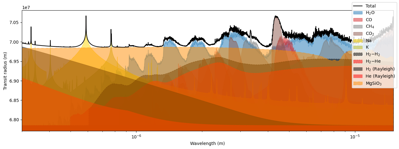
In petitRADTRANS, it is possible to plot the opacity contributions of a spectrum using the plot_opacity_contributions function.

[9]:

from petitRADTRANS.plotlib import plot_opacity_contributions

We can use the above transmission spectrum parameters.

[10]:

opacity_contributions = plot_opacity_contributions(
    atmosphere,
    mode='transmission',  # can also be 'emission'
    fill_below=True,  # if False, contributions are represented as cruves instead as a filled area
    x_axis_scale='log',  # 'linear' by default
    temperatures=temperatures,
    mass_fractions=mass_fractions,
    mean_molar_masses=mean_molar_masses,
    reference_gravity=reference_gravity,
    planet_radius=planet_radius,
    reference_pressure=reference_pressure,
)

Generating temporary Radtrans object with 'line_species': 'H2O'
Loading Radtrans opacities...
Loading line opacities of species 'H2O' from file '/home/dblain/petitRADTRANS/input_data/opacities/lines/correlated_k/H2O/1H2-16O/1H2-16O__HITEMP.R1000_0.1-250mu.ktable.petitRADTRANS.h5'... Done.
Successfully loaded all line opacities
Successfully loaded all opacities
Loading Radtrans opacities...
Loading line opacities of species 'H2O' from file '/home/dblain/petitRADTRANS/input_data/opacities/lines/correlated_k/H2O/1H2-16O/1H2-16O__HITEMP.R1000_0.1-250mu.ktable.petitRADTRANS.h5'... Done.
Successfully loaded all line opacities
Successfully loaded all opacities
Generating temporary Radtrans object with 'line_species': 'CO-NatAbund'
Loading Radtrans opacities...
Loading line opacities of species 'CO-NatAbund' from file '/home/dblain/petitRADTRANS/input_data/opacities/lines/correlated_k/CO/C-O-NatAbund/C-O-NatAbund__HITEMP.R1000_0.1-250mu.ktable.petitRADTRANS.h5'... Done.
Successfully loaded all line opacities
Successfully loaded all opacities
Generating temporary Radtrans object with 'line_species': 'CH4'
Loading Radtrans opacities...
Loading line opacities of species 'CH4' from file '/home/dblain/petitRADTRANS/input_data/opacities/lines/correlated_k/CH4/12C-1H4/12C-1H4__YT34to10.R1000_0.3-50mu.ktable.petitRADTRANS.h5'... Done.
Successfully loaded all line opacities
Successfully loaded all opacities
Generating temporary Radtrans object with 'line_species': 'CO2'
Loading Radtrans opacities...
Loading line opacities of species 'CO2' from file '/home/dblain/petitRADTRANS/input_data/opacities/lines/correlated_k/CO2/12C-16O2/12C-16O2__UCL-4000.R1000_0.3-50mu.ktable.petitRADTRANS.h5'... Done.
Successfully loaded all line opacities
Successfully loaded all opacities
Generating temporary Radtrans object with 'line_species': 'Na__Burrows'
Loading Radtrans opacities...
Loading line opacities of species 'Na__Burrows' from file '/home/dblain/petitRADTRANS/input_data/opacities/lines/correlated_k/Na/23Na/23Na__Burrows.R1000_0.1-250mu.ktable.petitRADTRANS.h5'... Done.
Successfully loaded all line opacities
Successfully loaded all opacities
Generating temporary Radtrans object with 'line_species': 'K__Burrows'
Loading Radtrans opacities...
Loading line opacities of species 'K__Burrows' from file '/home/dblain/petitRADTRANS/input_data/opacities/lines/correlated_k/K/39K/39K__Burrows.R1000_0.1-250mu.ktable.petitRADTRANS.h5'... Done.
Successfully loaded all line opacities
Successfully loaded all opacities
Generating temporary Radtrans object with 'gas_continuum_contributors': 'H2--H2-NatAbund__BoRi.R831_0.6-250mu'
Loading Radtrans opacities...
Loading line opacities of species 'H2O' from file '/home/dblain/petitRADTRANS/input_data/opacities/lines/correlated_k/H2O/1H2-16O/1H2-16O__HITEMP.R1000_0.1-250mu.ktable.petitRADTRANS.h5'... Done.
Successfully loaded all line opacities
Loading CIA opacities for H2--H2-NatAbund__BoRi.R831_0.6-250mu from file '/home/dblain/petitRADTRANS/input_data/opacities/continuum/collision_induced_absorptions/H2--H2/H2--H2-NatAbund/H2--H2-NatAbund__BoRi.R831_0.6-250mu.ciatable.petitRADTRANS.h5'... Done.
Successfully loaded all CIA opacities
Successfully loaded all opacities
Generating temporary Radtrans object with 'gas_continuum_contributors': 'H2--He-NatAbund__BoRi.DeltaWavenumber2_0.5-500mu'
Loading Radtrans opacities...
Loading line opacities of species 'H2O' from file '/home/dblain/petitRADTRANS/input_data/opacities/lines/correlated_k/H2O/1H2-16O/1H2-16O__HITEMP.R1000_0.1-250mu.ktable.petitRADTRANS.h5'... Done.
Successfully loaded all line opacities
Loading CIA opacities for H2--He-NatAbund__BoRi.DeltaWavenumber2_0.5-500mu from file '/home/dblain/petitRADTRANS/input_data/opacities/continuum/collision_induced_absorptions/H2--He/H2--He-NatAbund/H2--He-NatAbund__BoRi.DeltaWavenumber2_0.5-500mu.ciatable.petitRADTRANS.h5'... Done.
Successfully loaded all CIA opacities
Successfully loaded all opacities
Generating temporary Radtrans object with 'rayleigh_species': 'H2'
Loading Radtrans opacities...
Loading line opacities of species 'H2O' from file '/home/dblain/petitRADTRANS/input_data/opacities/lines/correlated_k/H2O/1H2-16O/1H2-16O__HITEMP.R1000_0.1-250mu.ktable.petitRADTRANS.h5'... Done.
Successfully loaded all line opacities
Successfully loaded all opacities
Generating temporary Radtrans object with 'rayleigh_species': 'He'
Loading Radtrans opacities...
Loading line opacities of species 'H2O' from file '/home/dblain/petitRADTRANS/input_data/opacities/lines/correlated_k/H2O/1H2-16O/1H2-16O__HITEMP.R1000_0.1-250mu.ktable.petitRADTRANS.h5'... Done.
Successfully loaded all line opacities
Successfully loaded all opacities

../../_images/content_notebooks_analysis_tools_33_1.png

It is also possible to exclude some opacity sources from the plot. The output dictionary opacity_contributions can be used as input.

The opacity_contributions directory can also be directly obtained from the Radtrans function calculate_contribution_spectra. That is, in this example, atmosphere.calculate_contribution_spectra.

[11]:

_ = plot_opacity_contributions(
    atmosphere,
    mode='transmission',
    exclude=['H2 (Rayleigh)', 'He (Rayleigh)', 'H2--H2', 'H2--He'],
    opacity_contributions=opacity_contributions,
    fill_below=True,
    x_axis_scale='log',
    temperatures=temperatures,
    mass_fractions=mass_fractions,
    mean_molar_masses=mean_molar_masses,
    reference_gravity=reference_gravity,
    planet_radius=planet_radius,
    reference_pressure=reference_pressure,
)

../../_images/content_notebooks_analysis_tools_35_0.png

Finally, their is a possibility to plot only the desired species. Colors and linestyles can be customised as well.

[12]:

_ = plot_opacity_contributions(
    atmosphere,
    mode='transmission',
    include=['Total', 'H2O', 'CO2', 'H2 (Rayleigh)'],
    colors={
        'Total': 'r',
        'line_species': {
            'H2O': 'aqua',
            'CO2': '#bcbd22'
        },
        'rayleigh_species': {
            'H2': 'purple'
        }
    },
    line_styles={
        'Total': '-.',
        'line_species': ':',
        'rayleigh_species': '--'
    },
    opacity_contributions=opacity_contributions,
    fill_below=True,
    x_axis_scale='log',
    temperatures=temperatures,
    mass_fractions=mass_fractions,
    mean_molar_masses=mean_molar_masses,
    reference_gravity=reference_gravity,
    planet_radius=planet_radius,
    reference_pressure=reference_pressure,
)

../../_images/content_notebooks_analysis_tools_37_0.png

Using `SpectralModel`#

To obtain this contribution plot from an existing model, it may be more parctical to use a SpectralModel. In that case, the function does not need any parameter input, as they are taken from the SpectralModel’s model parameters.

In the following example, we will generate a SpectralModel, then plot its contribution.

[13]:

from petitRADTRANS.spectral_model import SpectralModel

[14]:

spectral_model = SpectralModel(
    # Radtrans parameters
    pressures=np.logspace(-6, 3, 100),
    line_species=[
        'H2O',
        'CO-NatAbund',
        'CH4',
        'CO2',
        'Na__Burrows',
        'K__Burrows'
    ],
    rayleigh_species=['H2', 'He'],
    gas_continuum_contributors=['H2-H2', 'H2-He'],
    cloud_species=['MgSiO3(s)_crystalline__DHS'],
    wavelength_boundaries=[0.3, 15],
    # Model parameters
    temperature=temperatures,
    imposed_mass_fractions={  # using constant mass fractions with pressure
        'H2O': 1e-3,
        'CO-NatAbund': 1e-2,
        'CO2': 1e-4,
        'CH4': 1e-5,
        'Na__Burrows': 1e-4,
        'K__Burrows': 1e-6,
        'MgSiO3(s)_crystalline__DHS': 1e-6
    },
    filling_species={'H2': 37, 'He': 12},
    cloud_particles_mean_radii={'MgSiO3(s)_crystalline__DHS': 1e-4},  # (cm)
    cloud_particle_radius_distribution_std=2,  # 1 for a delta function
    reference_gravity=reference_gravity,
    planet_radius=planet_radius,
    reference_pressure=reference_pressure
)

[15]:

spectral_model.update_spectral_calculation_parameters(mode='transmission', **spectral_model.model_parameters)

[16]:

opacity_contributions = plot_opacity_contributions(
    spectral_model,
    mode='transmission',
    fill_below=True,
    x_axis_scale='log'
)

../../_images/content_notebooks_analysis_tools_43_1.png

Plotting opacities#

pRT can also be used to plot opacities. For this we can use the plot_radtrans_opacities() method, which we import here:

[17]:

from petitRADTRANS.plotlib import plot_radtrans_opacities

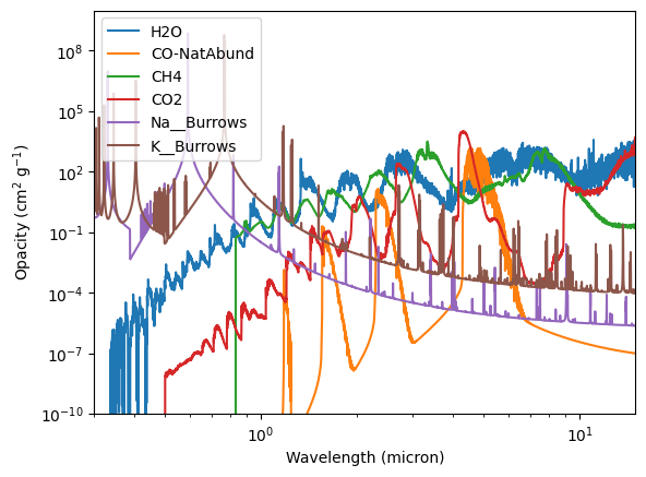
Next we plot the line opacities of the Radtrans object called atmosphere created above. This will assume (equal) abundances of 1 for the different species. Chemical equilibrium abundances are also possible, see below. Here we plot all line species of the Radtrans object, but also a subset of them is possible. Just give a list, for example ['H2O', 'CO-NatAbund'], instead of atmosphere.line_species, to the function. If you initialized your Radtrans object with line_opacity_mode='lbl' it will plot the high resolution opacities. For the default line_opacity_mode='c-k' it will plot the frequency-averaged opacities within the correlated-k frequency bins, like defined here for frequency bin \(i\):

\[\bar{\kappa}_i = \frac{1}{\Delta \nu_i} \int_{\nu_i - \Delta \nu_i/2}^{\nu_i + \Delta \nu_i / 2} \kappa(\nu)d\nu = \int_0^1 \kappa_i(g)dg\]

[18]:

plot_radtrans_opacities(
    atmosphere,
    atmosphere.line_species,
    temperature=1500.0,
    pressure_bar=0.1
)

plt.yscale('log')
plt.xscale('log')
plt.ylim([1e-10,1e10])
plt.xlim([0.3,15.])
plt.ylabel('Opacity (cm$^2$ g$^{-1}$)')
plt.xlabel('Wavelength (micron)')
plt.legend()

[18]:

<matplotlib.legend.Legend at 0x7f89770d7210>

../../_images/content_notebooks_analysis_tools_48_1.png

SpectalModel objects are also Radtrans objects, so they can be used with plot_radtrans_opacities, e.g.:

plot_radtrans_opacities(
    spectral_model,
    spectral_model.line_species,
    temperature=1500.,
    pressure_bar=0.1
)

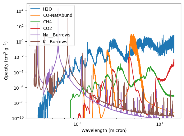
You can also use chemical equilibrium abundances for the relative weighting, here at C/O=0.55 (solar) and metallicity of 0 (solar). Not that it will notify you if it does not find a given species from atmosphere.line_species in the chemical abundance dictionary exactly, for example it will use the CO abundance for CO-NatAbund, etc.

[19]:

plot_radtrans_opacities(
    atmosphere,
    atmosphere.line_species,
    temperature=1500.0,
    pressure_bar=0.1,
    co_ratio=0.55,
    log10_metallicity=0.,
    mass_fractions='eq'
)

plt.yscale('log')
plt.xscale('log')
plt.ylim([1e-10,1e5])
plt.ylabel('Opacity (cm$^2$ g$^{-1}$)')
plt.xlabel('Wavelength (micron)')
plt.legend()

Loading chemical equilibrium chemistry table from file '/home/dblain/petitRADTRANS/input_data/pre_calculated_chemistry/equilibrium_chemistry/equilibrium_chemistry.chemtable.petitRADTRANS.h5'... Done.

[19]:

<matplotlib.legend.Legend at 0x7f8976d462d0>

../../_images/content_notebooks_analysis_tools_50_2.png

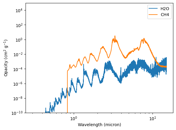
Or you choose the mass fractions of the absorber yourself. Note that plot_opas also supports all keyword arguments of matplotlib.plot() (here we use linestyle as an example).

[20]:

mass_fractions = {}
mass_fractions['H2O'] = 1e-6
mass_fractions['CH4'] = 1e-3

plot_radtrans_opacities(
    atmosphere,
    ['H2O', 'CH4'],
    temperature=1500.0,
    pressure_bar=0.1,
    mass_fractions=mass_fractions,
    linestyle = '--'
)

plt.yscale('log')
plt.xscale('log')
plt.ylim([1e-10,1e5])
plt.ylabel('Opacity (cm$^2$ g$^{-1}$)')
plt.xlabel('Wavelength (micron)')
plt.legend()

[20]:

<matplotlib.legend.Legend at 0x7f8976ea4750>

../../_images/content_notebooks_analysis_tools_52_1.png

If you set return_opacities=True it will return a dictionary with wavelengths and opacities for the various line absorbers you request, instead of plotting them. Then you can make a plot yourself (or other things)…

[21]:

opacities = plot_radtrans_opacities(
    atmosphere,
    ['H2O', 'CH4'],
    temperature=1500.0,
    pressure_bar=0.1,
    mass_fractions=mass_fractions,
    return_opacities=True
)

for species in opacities.keys():
    plt.plot(opacities[species][0], opacities[species][1], label=species)

plt.yscale('log')
plt.xscale('log')
plt.ylim([1e-10,1e5])
plt.ylabel('Opacity (cm$^2$ g$^{-1}$)')
plt.xlabel('Wavelength (micron)')
plt.legend()

[21]:

<matplotlib.legend.Legend at 0x7f8976d0c690>

../../_images/content_notebooks_analysis_tools_54_1.png

Getting mettalicity and elemental abundances from mass fractions#

In petitRADTRANS, it is possible to get a first, rough estimate of metallicity and element-over-hydrogen ratios using the mass_fractions2metallicity function.

The output is in regular scale, not in log scale.

An alternative function using volume mixing ratios,volume_mixing_ratios2metallicity, is also available.

The function estimates the metallicity from the given mass fraction dict. Elements and species not present in the mass fraction dict (but maybe present in an actual atmosphere) will not be accounted for, hence the results are necessarily a lower estimate of the actual atmospheric metallicity.

As with any metallicity obtained from atmospheric composition, the results are representative of the part of the atmosphere from which the species abundances have been inferred. It is not an estimation of the planet’s bulk metallicity, which would account for the metals in the core and deep atmosphere.

[22]:

from petitRADTRANS.chemistry.utils import mass_fractions2metallicity

[23]:

# The generated SpectralModel is used to have an atmospheric composition in which tbe sum of all mass fractions is 1
metallicity, h_ratios = mass_fractions2metallicity(spectral_model.mass_fractions, spectral_model.mean_molar_masses)

print(f"Z = {np.mean(metallicity):.2f} solar")

for dictionary in h_ratios.values():
    print(f"{dictionary['description']} = {np.mean(dictionary['relative to solar']):.2f} solar")

Z = 0.90 solar
He/H = 0.97 solar
C/H = 1.63 solar
O/H = 1.04 solar
Na/H = 3.13 solar
Mg/H = 0.00 solar
Si/H = 0.00 solar
K/H = 0.29 solar

Analysis tools

Contents

Analysis tools#

Transmission contribution functions#

Emission contribution functions#

Plotting opacity contributions#

Using Radtrans#

Using SpectralModel#

Plotting opacities#

Getting mettalicity and elemental abundances from mass fractions#

Using `Radtrans`#

Using `SpectralModel`#